1. Introduction |
Remote sensing techniques have been widely used since past four decades for inventorying, mapping and monitoring of natural resources. Diverse earth resources could be discriminated due to the dissimilarity among their spectral reflective properties. Recent trends in remote sensing technologies have lead to the improvements in sensor design, which have helped in acquiring the data with better spatial and spectral resolutions. These data could be analysed using either visual interpretation or automated digital processing techniques. Visual interpretation is based on interpretation keys such as tone, texture, shape, size and context. Compared to this, each individual pixel in an image is classified or grouped based on the spectral information in the digital image classification approaches. The supervised and unsupervised classification algorithms have been widely used for land use mapping exercises.
Algorithms based on supervised classification techniques, classify pixels considering the training site signatures as is done in Gaussian Maximum Likelihood classification (GMLC). This approach is based on probability density function associated with a particular signature (training site signatures). Pixels are assigned to most likely class based on a comparison of the posterior probability that it belongs to each of the signatures being considered. In contrast to this approach, Spectral Angle Mapper (SAM) compares each pixel in the image with every endmember for each class and assigns a ponderation value between 0 (low resemblance) and 1 (high resemblance). Endmembers are taken directly from the image and compared with signatures based on field experiments.
This endeavour evaluates the suitability of GMLC and SAM algorithms for land cover mapping (into agriculture, built up (urban/rural), forest, plantation/orchard, waste land/barren rock/sheet rock and water bodies) using superspectral data (MODIS) with spatial resolutions ranging between 250 m to 1 km and spectral resolution ranging from 7 to 36 bands with wavelength spread from 405 nm to 14.385 µm (covering visible and IR). This analysis was done using GRDSS (Geographic Resources Decision Support System) free and open source software (GRASS mirror site in India is at http://wgbis.ces.iisc.ac.in/grass). It has the capabilities to capture, store, process, display, organize, and prioritize spatial and temporal data. It serves as a decision support system for decision making and resource planning, with functionalities for raster analysis, vector analysis, modelling and visualization (Ramachandra T. V. & Kumar, Uttam., 2004, Ramachandra T. V. et al., 2004).
To compare two spectra, such as an image pixel spectrum and a library reference spectrum, the multidimensional vectors are defined for each spectrum and the angle between the two vectors is calculated. Smaller angles represent closer matches to the reference spectrum. If this angle is smaller than a given tolerance level, the spectra are considered to match, even if one spectrum is much brighter than the other (farther from the origin). Pixels further away than the specified maximum angle threshold are not classified (Lillesand et al., 2002). This is an easy and rapid method for mapping the spectral similarity of image spectra to reference spectra. SAM represses the influence of shading effects to accentuate the target reflectance characteristics (De Carvalho et al., 2000) and hence considered a very powerful classification method and functions well even with scaling noise. SAM is invariant to unknown multiplicative scalings, and consequently, is invariant to unknown deviations that may arise from different illumination and angle orientation (Keshava, et al., 2002). There is a high likelihood that angular information alone will provide good separation, when the pixel spectra from the different classes are well distributed in feature space. However, the spectral mixture or mixed pixels pose problems due to the assumption that endmembers represent the pure spectra of a reference material. This could happen even with the medium spatial resolution (30 m) images. SAM technique fails if the vector magnitude is important in providing discriminating information, which happens in many instances (Richards et al., 1996).
Girouard et al., (2004) validated SAM for geological mapping in Central Jebilet Morocco and compared the results between high and medium spatial resolution sensors, such as Quickbird and Landsat TM, respectively. The result showed that SAM of TM data can provide mineralogical maps that compare favourably with ground truth and known surface geology maps. Even though, Quickbird has a high spatial resolution compared to TM; its data did not provide good results for SAM because of low spectral resolution.
Gaussian maximum likelihood classifier assumes that the distribution of the cloud of points forming the category training data is Gaussian (normally distributed) and classifies an unknown pixel based on the variance and covariance of the category spectral response patterns. This classification is based on probability density function associated with a particular signature (training site). Pixels are assigned to most likely class based on a comparison of the posterior probability that it belongs to each of the signatures being considered. Under this assumption, the distribution of a category response pattern can be completely described by the mean vector and the covariance matrix. With these parameters, the statistical probability of a given pixel value being a member of a particular land cover class can be computed (Lillesand et al., 2002). GMLC can obtain minimum classification error under the assumption that the spectral data of each class is normally distributed. It considers not only the cluster centre but also its shape, size and orientation by calculating a statistical distance based on the mean values and covariance matrix of the clusters. A major drawback of this classifier is that large number of computations is required to classify each pixel. This is particularly true when either a large number of spectral channels are involved or a large number of spectral classes are to be differentiated. In such cases, the GMLC is much slower computationally than other algorithms. In addition, it is required to have the number of pixels per training set be between 10 times and 100 times as large as the number of sensor bands, in order to reliably derive class-specific covariance matrices.
An extension of the maximum likelihood approach is the Bayesian classifier, which applies two weighting factors to the probability estimate. First, the a priori probability, or the anticipated likelihood of occurrence for each class in the given scene is determined. Secondly, a weight associated with the cost of misclassification is applied to each class. Together, these factors act to minimize the cost of misclassification, resulting in a theoretically optimum classification. Most maximum likelihood classifications are performed assuming equal probability of occurrence and cost of misclassification for all classes. If suitable data exist for these factors, the Bayesian implementation of the classifier is preferable.
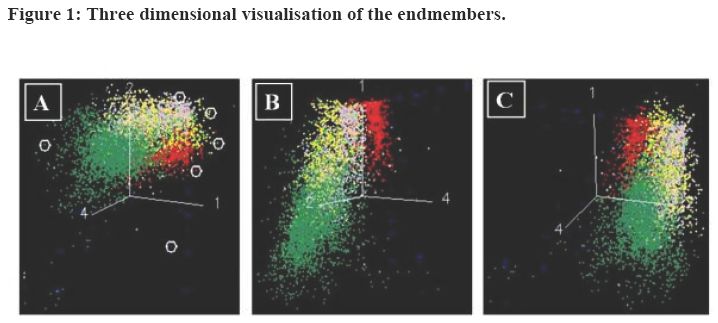
The reflected spectrum of a pure feature is called a reference or endmember spectrum. The training sets collected from the field were overlaid on the FCC of the image and a region of interest (ROI) was created, thus enabling direct selection of assumed pure pixels (endmembers) from the images. This was done for all classes (agriculture, built up, forest, plantation, waste land and water bodies) where a clear distinction between their pixels were possible. Scatter plots of the images also helped in locating some of the purest endmembers by taking the extreme corner pixels. A better match is obtained, if the endmember spectra are taken from the image cube under analysis. Finally, these spectra obtained by different methods were merged into six classes.
The spectra are the points in an n-dimensional scatter plot, where n is the number of bands. The coordinates of the points in n-space consist of n values that are simply the spectral reflectance values in each band for a given pixel. The distribution of these points in n-space was used to estimate the number of spectra and their spectral signatures, and provided an intuitive mean to understand the spectral characteristics of the land cover types. The spectral characteristics of the endmembers were analysed by plotting the endmembers and obtaining the Transformed Divergence matrix which showed a clear separability between the endmembers. These endmembers were then rotated using the n-dimensional visualiser. Snapshots of the visualisation are shown in figure 1. The endmembers are marked using white circles. It shows that the endmembers selected for the analysis are well separable and can be distinguished from each other.