 |
Land surface temperature with land cover dynamics: multi-resolution, spatio-temporal data analysis of Greater Bangalore |
 |
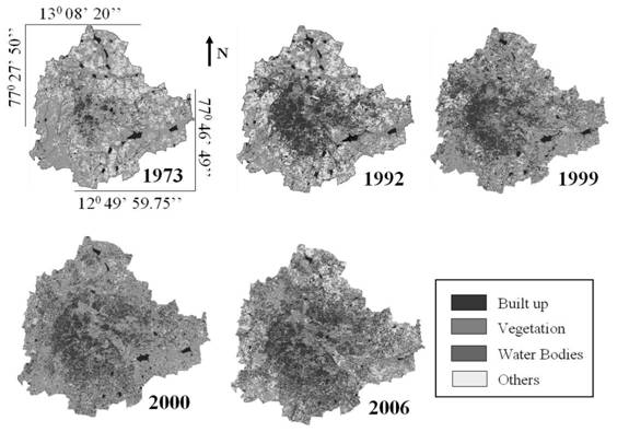
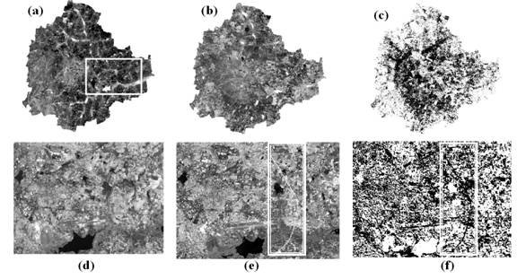
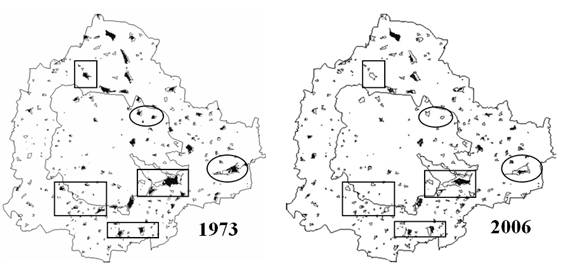
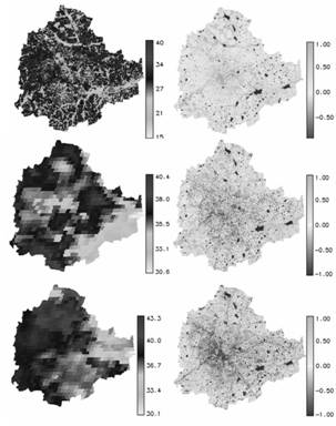
Results Temporal LU details are displayed in figure 2 and class statistics are listed in table 1. The classified images of 1973, 1992, 1999, 2000, 2002, 2006 and 2007 showed an overall accuracy of 72%, 75%, 71%, 77%, 60%, 73% and 55%. Accuracy assessment was performed which showed higher accuracy for high resolution data (~ 70-75% for Landsat and IRS LISS-III) and decreasing accuracy with coarse spatial resolution (~ 55-60% for MODIS). Figure 3 (a) – (f) depicts the LU change based on differencing techniques of PCA and TC. The disappearance of water bodies from 1973 to 2006 is given in Figure 4. 55% decline (from 207 to 93) in the number of water bodies and 61% decline in the spatial extent (of water bodies) is noticed from the temporal analysis. Validation was done considering training data and Google Earth image, covering approximately 15% of the study area. Then, pixels corresponding to urban category were extracted for further analysis. Figure 5 shows the LST and NDVI of Greater Bangalore in 1992, 2000 and 2007. The minimum (min) and maximum (max) temperature was 12 °C and 21 °C with a mean of 16.5±2.5 from Landsat TM (1992, winter). Similarly MODIS data of 2000 (summer) show the min, max and mean temperature of 20.23, 28.29 and 23.71±1.26 °C respectively. Corresponding values for 2007 (summer) are 23.79, 34.29 with a mean of 28.86±1.60 °C. LC wise NDVI and LST are listed in table 2.
TABLE 1. Greater Bangalore land cover statistics.
TABLE 2. NDVI and LST (°C) for respective land uses.
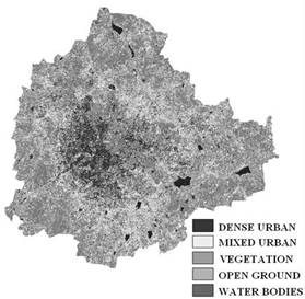
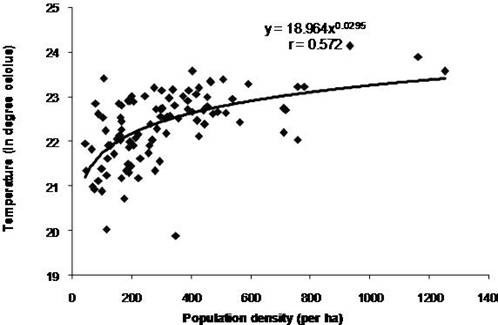
The relationship between LST and NDVI were investigated for each LC type through the Pearson’s correlation coefficient (CC) at a pixel level, which are listed in table 3. It is apparent that values tend to negatively correlate with NDVI for all LC types. NDVI values ranges from -0.05 to -0.6 (built up) and 0.15 to 0.6 (vegetation). Temporal increase in temperature with the increase in the number of urban pixels is noticed during 1992 to 2007 (63%) and ‘r’ confirms this relationship for the respective years. The decrease in vegetation is reflected by the respective increase in temperature. Further analysis is done by considering vegetation abundance. Landsat ETM+ (band 1, 2, 3, 4, 5 and 7) were unmixed to get the abundance maps of 5 classes (1) dense urban (commercial/industrial/residential), (2) mixed urban (urban with vegetation and open ground), (3) vegetation, (4) open ground and (5) water bodies. We considered only dense urban, mixed urban and vegetation abundance for further analysis as shown in figure 6. The min and max temperature from ETM+ data was 13.49 and 26.32 °C with a mean of 21.75±2.3. These abundance images were further analysed to see their contribution to the UHI by separating the pixels that contains 0-20%, 20-40%, 40-60%, 60-80% and 80-100% of the commercial/industrial/residential (dense urban), mixed urban and vegetation. Table 4 gives the mean and standard deviation (SD) of the LST for various LU. Application of decision based unmixing approach, systematically exploited the information from both the sources (sub-pixel class proportions and classified image based on training data collected from the ground) for achieving more reliable classification, shown in figure 7. Table 5 lists LC wise LST, NDVI and correlation coefficient. Relationship of population density with LST (Landsat ETM+) is evident in figure 8, which corroborate that the increase in LST is due to urbanisation and consequent increase in population.
TABLE 3. Correlation coefficients between LST and NDVI by LC type (significant at 0.05 level).
TABLE 4. Mean LST for different LC classes for various abundances.
TABLE 5. LST, NDVI and correlation coefficient for different LC classes.
TABLE 6. MMU sizes for different RS data sources used.
|
||||||||||||||||||||||||||||||||||||||||||||||||||||||||||||||||||||||||||||||||||||||||||||||||||||||||||||||||||||||||||||||||||||||||||||||||||||||||||||||||||||||||||||||||||||||||||||||||||||||||||