Data and Methods
Data:
Data used in the study are Landsat MSS (1973), TM (1992), IRS LISS-III MSS (1999), Landsat ETM+ (2000), IRS LISS-III (2006), MODIS 7 bands reflectance product (2002, 2007), MODIS Land Surface Temperature/Emissivity (V004 and V005): 8-Day, L3 Global 1km products (2000, 2007) and Google Earth (http://earth.google.com).
Study area:
Greater Bangalore the principal administrative, cultural, commercial, industrial, and knowledge capital of the state of Karnataka with an area of 741 km2 and lies between the latitudes 12°39’00’’ to 131°3’00’’ N and longitude 77°22’00’’ to 77°52’00’’ E. Bangalore city administrative jurisdiction was widened in 2006 by merging the existing area of Bangalore city spatial limits with 8 neighbouring Urban Local Bodies (ULBs) and 111 Villages of Bangalore Urban District. Thus, Bangalore has grown spatially more than ten times since 1949 (69 km2). Now, Bangalore (figure 1) is the fifth largest metropolis in India currently with a population of about 7 million (Ramachandra and Kumar, 2008).
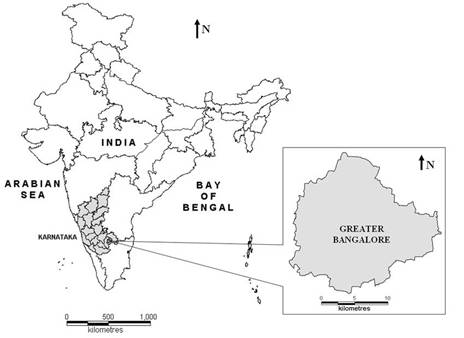
Figure 1. Study area – Greater Bangalore, India.
Methods:
- Land use analysis: This was done with Landsat data of 1973 (79 m spatial resolution), 1992 and 2000 (30 m), IRS LISS-III data of 1999 and 2006 (23.5 m) and MODIS data of 2002 and 2007 (250 m to 500 m spatial resolution) using supervised pattern classifiers based on Gaussian maximum likelihood (GML) estimation followed by a Bayesian statistical approach. This technique quantifies the tradeoffs between various classification decisions using probability and costs that accompany such decisions (Duda et al., 2000). It makes assumptions that the decision problem is posed in probabilistic terms, and that all of the relevant probability values are known with a number of design samples or training data collected from field that are particular representatives of the patterns to be classified. The mean and covariance are computed using maximum likelihood estimation with the best estimates that maximises the probability of the pixels falling into one of the classes. LU analysis considering temporal data (1973, 1992, 1999, 2000, 2002, 2006 and 2007) was done using the open source programs (i.gensig, i.class and i.maxlik) of Geographic Resources Analysis Support System (http://wgbis.ces.iisc.ac.in/grass).
- Change detection: LU change detection is performed by change/no-change recognition followed by boundary delineation on images of two different time periods. Pixels which show significant changes are checked and validated on the ground and the boundaries of the changed patches are category wise delineated. This is supplemented with visual interpretation and online digitisation. Many LU change detection techniques have been developed, but no single algorithm is suitable for all cases (Lu et al., 2004), as the implementation of change detection analysis is dependent on the data itself (Zhang and Zhang, 2007). Bi-temporal multispectral images have been analysed to understand LU dynamics through:
- Principal Component Analysis(PCA) – PCA has been an effective tool for change detection (Fung and LeDrew, 1987; Michener and Houhoulis, 1997). Major components of the time two (t2) data are subtracted from the corresponding components of the time one (t1) data to obtain differences related to changes in LU. This method provides a better result than simple image differencing when the radiometric differences between the two images are too large due to different imaging circumstances and cannot be effectively dealt with by the radiometric normalisation process (Zhang and Zhang, 2007). Landsat MSS (1973) and IRS LISS-III (2006) scenes having different radiometry were used with PCA to understand the overall changes across a period of 33 years.
- Tasseled Cap (TC) or Kauth-Thomas (KT) transformation – Here, multi-temporal TM and ETM+ data are transformed into the brightness-greenness-wetness space, then changed areas are generated by differencing the brightness (ΔB) and greenness (ΔG) values (Kauth and Thomas, 1976). Changes in brightness (ΔB) are associated with most LU changes, especially constructed related changes. TC results can be physically interpreted as its coefficients are predetermined and independent of each image scene, while PCA coefficients are not. However, for the purpose of simply detecting change/no-change areas, PCA is better than TC in many cases, although the physical interpretation is difficult. TC transformations were performed on Landsat TM (1992) and ETM+ (2000) data.
- Image differencing (ID) – ID is effective for identifying LU changes from visible and NIR band pairs acquired in similar circumstances (imaging conditions) using same sensor over two different time periods (Macleod and Congalton, 1998). IRS LISS-III (1999 and 2006) data was used to visualise the LU changes through ID.
- Derivation of LST from Landsat TM and Landsat ETM+: LST were computed (Weng et al., 2004) from TIR bands (Landsat TM and ETM+). Emissivity correction for the specified LC is carried out using surface emissivities as per Synder et al., (1998); Stathopoplou et al., (2007) and Landsat 7 science data user’s handbook (2008). The emmissivity corrected land surface temperature (Ts) are computed as per Artis and Carnahan (1982)
|

|
….. (Equation 1) |
where, λ is the wavelength of emitted radiance for which the peak response and the average of the limiting wavelengths (λ = 11.5 μm) (Markham and Barker, 1985) were used, ρ = h x c/σ (1.438 x 10⁻² mK), σ = Stefan Bolzmann’s constant (5.67 x 10⁻⁸ Wm-2K-4 = 1.38 x 10⁻²³ J/K), h = Planck’s constant (6.626 x 10⁻³⁴ Jsec), c = velocity of light (2.998 x 10⁸ m/sec), and ε is spectral emissivity.
- LST from MODIS: MODIS LST/Emissivity 16-bit unsigned integer data with 1 km spatial resolution are multiplied by a scale factor of 0.02 (http://lpdaac.usgs.gov/modis/dataproducts.asp#mod11) and are converted to degree Celsius.
- NDVI from Landsat TM, ETM+ and MODIS: NDVI was computed using visible Red (0.0.63 – 0.69 μm) and NIR (0.76 – 0.90 μm) bands of Landsat TM (1992)/ETM+ (2000) and Red (0.62 – 0.68 microns) and NIR (0.77 – 0.86 microns) bands of LISS-III data of 2006.
- Estimation of abundance maps: Linear unmixing method was adopted for solving the mixed pixel problem as the spectral radiance measured by a sensor consists of the mixture of radiances reflected in proportion to the sub-pixel area covered (Kumar, U., et al., 2008). Endmembers corresponding to pure pixels are given by the reference spectra of each of the individual pure materials. Spectra corresponding to sub-pixel areas in a pixel are assumed to be linearly independent, and the target pixel spectra are a combination of these spectra (which is proportional to respective LC in a pixel). The spectrum measured by a sensor is a linear combination of the spectra, therefore,
|

|
….. (Equation 2) |
where n = the number of distinct LU classes; yi = Spectral reflectance of respective pixels in a band; aij = Spectral reflectance of the jth component in the pixel for ith spectral band; xj = Proportion value of the jth component in the pixel; j = 1, 2, 3 ... n (number of land classes assumed); i = 1, 2, 3 ... m (number of multispectral bands) and ei = error term for the ith spectral band. The error term (ei) is due to the assumption made that the response of each pixel in any spectral wavelength is a linear combination of the proportional responses of each component. Assuming that the error term is 0, equation 2 can be written as
AX = Y ….. (Equation 3)
where A is a m x n matrix (a11, a12, …, amn), X is a n x 1 vector (x1, x2, …, xn) and Y is a n x 1 vector (y1, y2, …, yn) written as,
|

|
….. (Equation 4) |
|

|
….. (Equation 5) |
Equation 5 gives the Constrained Least Squares (CLS) estimate of the abundance expressed in terms of matrix A, X and Y. The reflected spectrum of a pure feature is called a reference or endmember spectrum. Endmembers are extracted using scatter plot or through automatic endmember extraction techniques (Kumar, U., et al., 2008).
- LC derivation from abundance values along with training polygons using Bayesian classification: Abundances of each category (pixel wise) is used as a prior probability of the class. In the Baye's classifier for the multispectral data, the posterior probability of the class given the observation is computed by multiplying the prior probability of the class with the conditional probability P(x|k), where x denotes the multispectral observation vector and k any class. The class label assigned to the pixel is
|

|
….. (Equation 6) |
|