2. Methods

2.1 Orthogonal Subspace Projection (OSP) – When the object size is smaller than the pixel resolution, e.g., houses/buildings in a 250 m (or 500 m or 1 Km) spatial resolution on the earth's surface, each pixel usually contain contributions from more than one class, and are termed mixed pixels. Standard classification techniques, which attribute a single class to the entire pixel, are therefore inappropriate to low resolution satellite images. This motivates the development of algorithms which unmix the coarse data or, in other words, perform classification at a sub-pixel level. The main objective is to find out the proportion of each category in a given pixel, or in other words, unmix the pixel to identify the categories present within the pixel. In order to address this problem, unmixing techniques have been developed to exploit sub-pixel level information for image analysis (Shimabukuro and Smith, 1991), where sub-pixel class composition is estimated through the use of techniques, such as linear mixture modelling (Kumar et al., 2008), supervised fuzzy-c means classification (Foody and Cox, 1994) and artificial neural networks (Kanellopoulos et al., 1992), etc.

Linear unmixing is based on an assumption that the spectral radiance measured by the sensor consists of the radiances reflected collectively in proportion to the sub-pixel area covered by each material. Let K be the number of bands in the multispectral/superspectral data set, and P, the number of distinct classes of objects in the physical scene. Associated with each pixel is a K-dimensional vector y whose components are the gray values corresponding to the K bands. Let E = [e₁, e₂,…, e_P], where {e_i} is a column vector representing the spectral signature of the i^th target material or category. The column vectors of the K x P matrix E are called end-members. For a given pixel, the abundance fraction of the p^th target material present in a pixel is denoted by α_P, and these values are the components of the P-dimensional abundance vector α. Assuming the linear mixture model, the observation vector y is related to E by

                                                                                                                            (1)

where  accounts for the measurement noise. We further assume that the components of the noise vector  are zero-mean random variables that are independent and identically distributed. Therefore, the covariance matrix of the noise vector is , where  is the variance, and I is K x K identity matrix. The conventional approach (Nielsen, 2001) to extract the abundance values is to minimise , and the estimate for the abundance is

                                                                                                                       (2)

which is termed as the Unconstrained Least Squares (ULS) estimate of the abundance. Imposing the sum-to-one constraint on the abundance values while minimising , gives the Constrained Least Squares (CLS) estimate of the abundance as,

                                                                                                           (3)

where,

                                                                                                          (4)

Chang (2005), recently came up with a classification technique referred to as OSP based on two aspects: 1) how to best utilize the target knowledge provided a priori and 2) how to effectively make use of numerous spectral bands. Briefly, the technique involves (i) finding an operator which eliminates undesired spectral signatures, and then (ii) choosing a vector operator which maximises the SNR of the residual spectral signature. In order to find the abundance of the p^th target material (α_P), let the corresponding spectral signature of the desired target material be denoted as d. The term Eα in equation (1) can be rewritten to separate the desired spectral signature d from the rest as:

                                                                                                                      (5)

where r contains the abundance of the rest of the end-members, and R is a K x P - 1 matrix containing the columns of E except for the column vector d. We rewrite (1) as

.                                                                                                                 (6)
The interfering signatures present in R can be removed from the above equation by the operator,

                                                                                                            (7)

which can be used to project the vector y into a space orthogonal to the space spanned by the interfering spectral signatures. Therefore, operating on y with P, and noting that PR = 0, we get

.                                                                                                                    (8)

The next step is to find an operator w^T which maximizes the SNR given by

                                                                             (9)

Maximizing the SNR leads to the generalized eigenvalue problem:

.

The eigenvector corresponding to the maximum eigenvalue of the above eigenvalue problem is the vector w that we are looking for. It can be shown that the w which maximises the SNR is given by

w = kd .                                                                                                                                    (10)

Therefore, an optimal estimate of α_p is given by

                                                                                                                        (11)

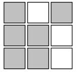
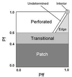
In the absence of noise, the estimate matches with the exact value as given in equation (6). The value of α is the abundance of the p^th class (in an abundance map) ranging from 0 to 1 in any given pixel. 0 indicates absence of a particular class and 1 indicates full presence of that class in that particular pixel. There are as many abundance maps as the number of classes. Intermediate values between 0 and 1 may represent a fraction of that class. For example, 0.4 may represent 40% presence of a class in an abundance map and the remaining 60% could be some other class. If the objective is to map the impervious surface, then OSP renders an impervious surface abundance map, where each abundance pixel shows the proportion of impervious material (buildings/houses/roads/paved surfaces, etc.) in that pixel.      

2.2 Forest fragmentation – Forest fragmentation is the process whereby a large, continuous area of forest is both reduced in area and divided into two or more fragments. The decline in the size of the forest and the increasing isolation between the two remnant patches of the forest has been the major cause of declining biodiversity (Tucker and Richards, 1983; Turner, 1990; Meyer and Turner, 1994; Houghton, 1994; Hurd, et al., 2001). The primary concern is direct loss of forest area, and all disturbed forests are subject to “edge effects’ of one kind or another. Forest fragmentation is of additional concern, insofar as the “edge effect” is mitigated by the residual spatial pattern (Forman and Godron, 1986; Turner, 1989; Levin, 1992)

Land cover (LC) maps indicate only the location and type of forest, and further analysis is needed to quantify the forest fragmentation. For calculating fragmentation statistics and for defining the total extent of forest and its occurrence as adjacent pixels, fixed-area windows surrounding each forest pixel is used. This information is used to classify the window by the type of fragmentation. The result is stored at the location of the centre pixel. Thus, a pixel value in the derived map refers to between-pixel fragmentation around the corresponding forest location. As an example (Ritters et al, 2000), the measurements are illustrated in figure 1 and 2. Let Pf be the proportion of pixels in the window that are forested. Pff is defined as the proportion of all adjacent (cardinal directions only) pixel pairs that include at least one forest pixel, for which both pixels are forested. Pff estimates the conditional probability that, given a pixel of forest, its neighbour is also forest. The six fragmentation model that identifies six fragmentation categories are: (1) interior, for which Pf = 1.0; (2), patch, Pf < 0.4;  (3) transtitional, 0.4 < Pf < 0.6; (4) edge, Pf > 0.6 and Pf – Pff > 0; (5) perforated, Pf > 0.6 and Pf – Pff < 0, and (6) undetermined, Pf > 0.6 and Pf = Pff.

Figure 1: Computation of Pf and Pff for a 3 x 3 grid of pixels. Forest pixels are shaded and nonforest pixels are not shaded. Here, six of the nine pixels are forested and so Pf equals 6/9=0.67. Considering pairs of pixels in cardinal directions, the total number of adjacent pixel pairs is 12, and of these, 11 pairs include at least one forested pixel. Five of those 11 pairs are forest-forest pairs, so Pff equals 5/11 = 0.45.

When Pff is larger than Pf, the implication is that forest is clumped; the probability that an immediate neighbour is also forest is greater than the average probability of forest within the window. Conversely, when Pff is smaller than Pf, the implication is that whatever is nonforest is clumped. The difference (Pf-Pff) characterizes a gradient from forest clumping (edge) to nonforest clumping (perforated). When Pff = Pf, the model cannot distinguish forest or nonforest clumping. The case of Pf = 1.0 (interior) represents a completely forested window for which Pff must be 1.0.

Figure 2 : The model used to identify forest fragmentation categories from local measurements of Pf and Pff in a fixed area window (adapted from Ritters et al, 2000).

Based on the fragmentation model, a state of forest fragmentation index is computed (Hurd et al., 2002). This has two parts: (1) Total forest proportion (TFP) and Forest continuity (FC). TFP provides a basic assessment of forest cover in a region ranging from 0 to 1. FC value examines only the forested areas within the analysis region. It measures specifically utilises the results from the forest fragmentation model.

                                                                                               (12)

                                          (13)

Weighted values for the weighted forest area (WFA) are derived from the median Pf value for each fragmentation class as given by equation below:

                                       (14)

The rationale is that, given two regions of equal forest cover, the one with more interior forest would have a higher weighted area, and thus be less fragmented. To separate further regions based on the level of fragmentation, the weight area ratio is multiplied by the ratio of the largest interior forest patch to total forest area for the region. FC ranges from 0 to 1.

2.3 Urban Growth Characterisation – An urban growth model has spatially detailed data with fine spatial grain, examines the whole landscape and helps in regional planning, assesses urban growth in all areas, avoids spatial averaging, maintains spatial pattern and configuration, and is consistent over time. The urban growth model used here in based on the modified forest fragmentation model developed by Ritters et al., (2000) and described earlier. The urban growth model uses urban and non-urban classes to create fragmentation image instead of forest and non-forest in forest fragmentation model (Civco et al., 2002). Input data consist of multi-dates LC with a minimum of three classes; urban (developed), non-urban (non-developed), and water. Instead of using a forest versus non-forest binary image to create a forest fragmentation map, the first step of the urban growth model uses a non-developed versus developed image to create a “non-developed” fragmentation image. The single date fragmentation map consist of three “fragmented” classes that are combinations of the five classes previously described (interior, patch, transitional, edge and perforated). The first is interior, which occurs when all pixels in a 3 x 3 window are non-developed. The second class is perforated, which occurs when between 60 % and less than 100 % of pixels in a 3 x 3 window are non-developed. The final class is patch, which occurs when fever than 60 % of pixels in a 3 x 3 window are non-developed. Two dates of fragmentation maps are used to create change map. There are three types of change classes – the first type consists of no change classes (including developed, water and interior), the second type includes improbable changes, likely due to classification error, and the third type consists of classes that represent urban growth. The classes that indicate urban growth are outlines in table 1 along with their corresponding urban growth classes. The change classes determine the type of urban growth.

Table 1: Change classes that represent urban growth and the corresponding growth types

Infill is the development of a small area surrounded by existing developed land. Expansion is the spreading out of urban LC from existing developed land. Outlying growth is an interior pixel that changes to developed, and is further classified as either isolated, linear branching, or clustered branching. Their distinction is made using a set of rules. An isolated growth is defined as a new, small area of construction surrounded by non-urban land and some distance from other developed areas. A linear branching growth is a road, corridor, or linear development surrounded by non-urban land and some distance from other urban areas. A clustered branching growth is indicative of a new, large and dense development in a previously undeveloped area. The urban growth model produces an urban growth map, which consists of five types of growth as well as developed land, water, and non-developed land.