VI. RESULTS |
LC analysis using LISS-III MSS data
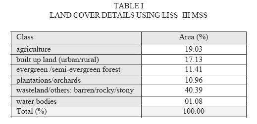
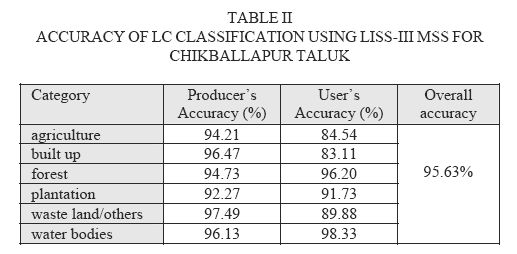
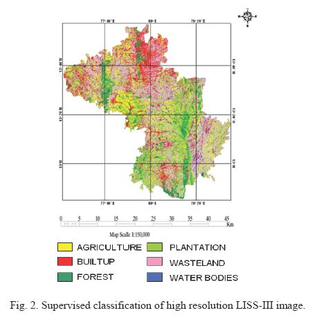
The class spectral characteristics for six LC categories using LISS-III MSS bands 2, 3 and 4 were obtained from the training pixels spectra to assess their inter-class separability and the images were classified with training data uniformly distributed over the study area collected with pre calibrated GPS (Fig. 2). This was validated with the representative field data (training sets collected covering the entire district and a detailed validation in Chikballapur Taluk covering ~ 15% of the study area) and the LC statistics are given in Table I. Producers, users, and overall accuracy computed are listed in Table II. A kappa (k) statistics of 0.95 was obtained indicating that the classified outputs are in good agreement with the ground conditions to the extent of 95%.
Classification errors can occur when the signal of a pixel is ambiguous, perhaps as a result of spectral mixing, or due to overlap of spectral reflectance (as in the case of certain agriculture and horticulture crops) or when the signal is produced by a cover type that is not accounted for in the training process. Another possible source of error may be due to the temporal difference in training data collection and image acquisition.
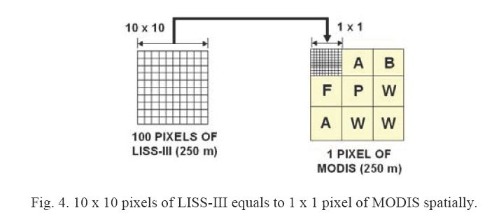
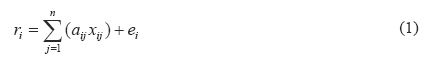
Here each pixel spectrum of an image is modeled as a linear combination of a finite set of known components (or endmembers) given by (1)
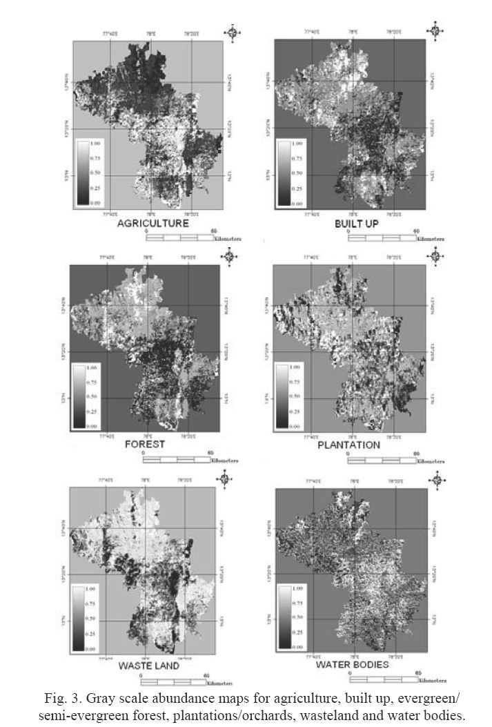
Visual inspection as well as accuracy assessment of abundance images corresponding to each endmember showed that the CLSU algorithm maps LC categories spatially and proportionally similar to supervised classified image of LISS-III. The proportions of the endmembers in these images (Fig. 3) range from 0 to 1, with 0 indicating absence of the endmember and increasing value showing higher abundance.
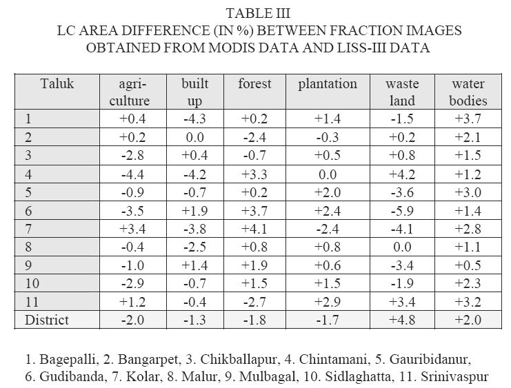
Bright pixels represent higher abundance of 50% or more stretched from black to white. Errors were found due to confusion between agriculture and horticulture (plantation) in the central regions and built up and wasteland in northern regions of the district. Overall, the distribution and abundance values of other classes are comparable within ±6 % to the classified outputs of LISS-III. There are many areas where proportions of agriculture are properly identified, mainly in the western central portion of the study area. However, there is also underestimation of agriculture in the south-central region due to errors of commission and omission.
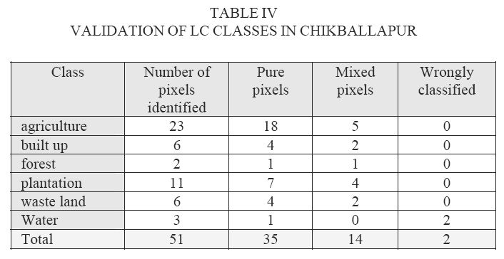
A total of 51 pixels with respect to the six LC classes were verified, and the result is tabulated in Table IV. The validation indicates that 35 pure and 14 mixed were correctly classified. Two pixels were misclassified; belong to water bodies which constitute < 1% of the total area.