V. MATERIALS AND METHODS |
MODIS data with atmospheric corrections, also known as the MOD 09 Surface Reflectance 8-day L3 global product at 250 m (band 1 and 2) and 500 m (bands 3 to 7) in Hierarchical Data Format (HDF), were downloaded from the Earth Observing System Data Gateway [31]. They are radiometrically corrected, fully calibrated and geolocated radiances at-aperture for all MODIS spectral bands and are processed to Level 3G. The spectral range is from 0.45 to 2.15 µm [28]. IRS - 1C/D LISS-III MSS (Multi Spectral Scanner) data in 3 bands (G, R and NIR, 0.52 to 0.86 µm) with a spatial resolution of 23.5 m were purchased from NRSA (National Remote Sensing Agency), Hyderabad.
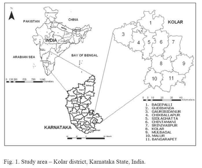
The Kolar district in Karnataka State, India, located in the southern plain regions (semi arid agro-climatic zone) and extending over an area of 8238 km2 between 77°21' to 78°35' E and 12°46' to 13°58' N, was chosen for this study (Fig. 1). Kolar is divided into 11 taluks for administration purposes. Rainfall occurs mainly during southwest and northeast monsoon seasons. The average population density of the district is about 209 persons/km2 [32]. The study area is mainly dominated by agricultural land, built up (urban/rural), evergreen/semi-evergreen forest, plantations/orchards, waste lands and water bodies. There are a few other LC classes (barren/rock/stone/others) that have very limited ground area proportions and are unevenly scattered among the major six classes, and were grouped under the waste land category. Fig. 1. Study area Kolar district, Karnataka State, India.
The study involved creation of base layers, such as district, taluk and village boundaries, road network, etc. from the Survey of India (SOI) topographic maps of scale 1:250000 and 1:50000. The LISS-III bands were geo-registered using ground control points (GCPs). LISS-III bands were resampled to 25 m, which helped in pixel level comparison of abundance maps obtained by unmixing MODIS data with LISS-III classified map. This was followed by cropping and mosaicing of data corresponding to the study area from the image scenes. Supervised classification was performed on LISS-III MSS data using a Gaussian Maximum Likelihood Classifier (GMLC) followed by accuracy assessment. The MODIS data were geo-corrected with an error of 7 meters with respect to LISS-III images. The 500 m resolution bands 3 to 7 were resampled to 250 m using nearest neighbourhood technique (with Polyconic projection and Evrst 1956 as the datum). Minimum Noise Fraction (MNF) components were derived from the 7 bands to reduce noise and computational requirements for subsequent processing. Endmembers were extracted directly from the data without using existing spectral libraries through:
(a) Pixel Purity Index (PPI) with the MNF components,
(b) Scatter Plot,
(c) N-Dimensional Visualization and
(d) Collected training data - training polygons (= 250 x 250 m) of homogenous patches corresponding to MODIS pure pixels were collected in the study area, thus enabling direct selection of assumed pure pixels from the images.
The spectral characteristics of the endmembers were analysed by plotting them and analysing their separability using a Transformed Divergence matrix. It shows that the endmembers selected for the analysis are separable and can be distinguished from each other. The abundance maps were generated via constrained linear unmixing of MODIS data. Accuracy assessment was done for the abundance maps: LC percentages were compared at boundary level and at pixel level with a LISS-III classified map and also with ground truth data which is discussed later (Accuracy assessment).