| Back | Paper1 | Paper2 | Next Session |
SESSION-1 Limnology
PAPER-1 Principles of modern Liminology - Jack R. Vallentyne
As a group, geologists are engaged in the perhaps the morbid (though awe-inspiring) study of the past. It is therefore a pleasure to add a little of the present to this symposium, for it is in that sense that the word modern has been used in the title. We shall have a glimpse at the goings-on within a lake not so much in terms of factual material as in terms of principles and generalities. In order to do this I will discuss the lake in terms of simple physics and the over-all metabolism. When I am through you will probably find yourself no better equipped to undertake the study of a lake than you are now, though you may have a general understanding of the lake in terms of processes. Let us begin by examining the physics of a lake. With this basic framework we can then turn to the study of interactions of biological and chemical factors (metabolism).
| Part I : The Physical Background | up | previous | next | last |
It is with great interest that one scans the title of Sir Douglas Mawson's paper [1], “Occurrence of water in Lake Eyre, South Australia”. It is an important title, because if we look at it out of context, it focuses attention on the fact that a lake is completely composed of water (The title actually refers to the presence of water in a formerly dry lake basin). It stresses that water should be the first study of the limnologist. Most often, however, it is the last, for the beginning student is more attracted to the diversity of aquatic life: the whirligig beetles, bottom living insects, fish and other fantastic forms of life.
The main point to be clear on is that water is not a single molecular substance. In the first place, it is a mixture of hydrogen and deuterium (to a lesser extent also tritium) isotopes in combination with isotopes of oxygen. However, this variable isotopic combination is not peculiar to water as a chemical entity for it is characteristic of most natural organic substances. The peculiar property is that water molecules (H 2 O) by virtue of their dipolar nature, interact to form quasi-stable polymers. The nature of associations between water molecules is little understood, but the evidence for association can hardly be disputed (see Dorsey [2] for a discussion of the subject). The nature of the linkages varies with temperature and pressure in a complex fashion. As a result it is customary to find that water shows peculiar, non-linear relationships to changing physical conditions. Although there is no conclusive agreement, it would seem that the new equilibrium states of association are assumed instantaneously with change in temperature or pressure.
Water has the highest specific heat of all substances except liquid hydrogen and lithium at high temperatures. It is this high absorption capacity for heat, which permits the local modification of climate by a water body. But the most interesting property of water to a limnologist is the parabola-like variation of density with temperature, water reaching a maximum density at 3.98°C under a pressure of one atmosphere.
If the pressure on water is increased, as it is with depth in a lake (pressure increases one atmosphere for every 10 meters depth), water is compressed to a small but measurable extent. This increased density in situ may lead to a lowering of the temperature of maximum density in the waters of deep lakes as Münster-Strom [3] has indeed shown. The depression is small. It can only be measured in terms of a fraction of a degree even for the deepest of all lakes, Lake Baikal, Russia (1706 meters or about one mile deep).
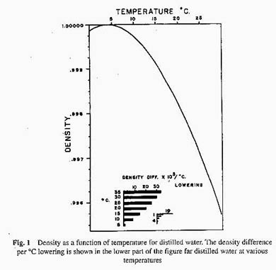
Let us start with a lake, about 15 meters maximum depth, located in north temperate latitudes. At some time during early spring, after the ice cover has disappeared the temperature will be approximately 4 ° C throughout the lake. As the surface water becomes heated from above by sun's radiation, temperature stratification will develop, dividing the lake into a warm upper part and a lower cold part. Let us further assume that salinity (the content of dissolved salts) is uniform throughout the lake, and that the only factor regulating the density of water is its temperature. Figure 1 shows how the density of distilled water varies with temperature. For our purposes it is more profitable to examine the difference in density between water at a given temperature and water at a temperature 1 ° C lower. We shall call this the density difference per degree centigrade lowering. The magnitude of this density difference for water of different temperatures is shown in the lower part of Figure 1. One can see that the density difference per degree lowering increases as the temperature departs from 4 ° C, either above or below. In order to mix fluids of differing density, physical work must be performed, just as is the case when mixing cream in a bottle of milk. All other factors constant, the amount of work that must be done is proportional to the difference in density.
Thus, forty times as much work is required to mix layered water masses at 30 and 29 ° as the same masses at 5 and 4 ° , because the density difference is approximately forty times greater. Before pursuing the matter further, we must consider a phenomenon, which the physical chemist knows under the title Lambert's law. This law states that the light absorbed by a solution increases exponentially with the light path through the solution. For light of wavelength 0.75 m and a column of water 1m long, only 10% passes through – 90% is absorbed. If the length of the water column is increased to 2 meters, 1% passes through and 99% is absorbed. Since much of the sun's radiation is of this wavelength (0.75 m ) or higher (infrared radiation), it will be clear that the uppermost two meters of the lake water absorb half of the sun's radiation. It is this absorbed radiation that is responsible for heating of the water.
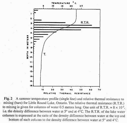
Now we may examine a typical temperature-depth curve for a lake, such as the solid line shown in Figure 2. If what we had said up to now were true, we should expect quite a different type of temperature curve, one in which the temperature decreased rapidly with depth, particularly in the uppermost meter or two. What is wrong? We have forgotten to mention one factor of prime importance; that the surface waters, which are heated by the sun, are mixed at the same time by the wind. The wind's work is important in heat transfer. We can now begin to see how this operates in the lake to produce the observed temperature curves. With regard to Figure 2, let us divide the lake into three water masses: the epilimnion of warm isothermal water, the hypolimnion of cold isothermal water, and the intermediate thermocline where the temperature declines rapidly with depth. The temperature curve shown in Figure 2 reflects the influence of sun in warming surface waters and the work of the wind in pushing part of the warmed surface water down to a depth of 10 meters in the lake. There appears to be some sort of barrier in the region of the thermocline, which prevents transfer of heated water to the deeper regions. What is the nature of this barrier? Before this question can be considered, we must return to a consideration of density.
As a general rule we can say that temperature is the most important factor regulating the density of lake water, though I shall mention an exception in a minute. Let us divide the temperature curve shown in Figure 2 into ½ meter intervals and calculate the densities of water at the top and bottom of each ½ meter interval (calculated from knowledge of the temperatures). What we are going to do is calculate the relative resistance to mixing offered by each ½ meter interval. A ½ meter column with a temperature gradient from 5 ° above to 4 ° below will be used as the standard. We shall define such a column as having one unit of relative thermal resistance to mixing. From knowledge of the density difference in the standard column and those in the ½ meter columns of lake water, one may calculate (Following Birge [4]) the relative thermal resistance to mixing offered by each ½ meter depth interval. The values are shown by solid bars in Figure 2. There are two instructive points of interest. Note first of all how a barely perceptible temperature difference (0.1 ° C) in the warm water at the surface leads to a large increase in the resistance to mixing, and secondly how the resistance reaches a maximum which lies slightly above the inflection point of the temperature curve. You should be able to explain these observations from what we have already said regarding density difference per degree lowering as related to temperature. The mixing barrier in the thermocline region is thus due to the large density differences there, induced solely by the depth-declining temperature.
As a result of the temperature-dependent stratification of density, the water in the epilimnion circulates freely; but just as the walls of the lake deflects these currents down on the leeward side, so does the mixing barrier in the thermocline deflect them horizontally in the opposite direction to the surface movement. Any attempt on the part of the wind to mix epilimnetic with thermocline water in the lake would result in an increased density gradient in the thermocline region, and thus an increased barrier to mixing. The thermocline tends to maintain itself by this self-regulating mechanism, unless certain other conditions are changed.
The depth of the thermocline in a lake depends on a number of factors, not the least of which is exposure to the wind. In very windy areas, a lake as deep as 26 meters may be without a thermocline. Also, depending on the heat content of incoming water (inlets, springs, rain) the thermocline may be depressed or raised.
The relative importance of the sun and wind in heating the lake varies with the season. In the spring when the water is cool and easily mixed, the radiation from the sun is low and the wind is the effective agent in heating, but as summer approaches the sun's intensity increases and the wind becomes less effective because of its inability to work against greater density gradients in the water. With the approach of autumn, the lake loses heat to its surroundings. Convection currents set up by the cooled surface waters, together with the work of the wind, cause the lake water to assume the uniform low temperature characteristic of springtime.
In deep tropical lakes it is not uncommon to find surface temperatures of 30 ° and bottom temperatures, not of 4 ° , but of 20-25 ° C. This introduces another principle: the temperature of the hypolimnion cannot be lower than the mean air temperature for the coldest period at the time of previous circulation (complete mixing of all the water in the lake). In terms of stability to mixing by the wind, tropical lakes sometimes differ from the hypothetical lake that we have been describing, in spite of the small temperature difference between the top and the bottom. The reason is again due to the great density difference per degree lowering at high temperatures (see Fig.1).
Occasionally, lakes are found that have temperature curves not unlike those shown in Figure 2, but with increases of several degrees in the deepest water. Something is obviously the matter, for if you have followed our arguments so far, you will appreciate that the layering of cold above warm water is a physically unstable situation. The trouble is that we have forgotten a previous assumption: that of constant salinity. In these peculiar lakes (termed meromictic or partially circulating lakes in distinction to our theoretical holomictic lake) the bottom water never or rarely circulates with the overlying water.
Frey [5] has recently studied a European lake (Längsee) in which the water in the bottom monimolimnion has not mixed with the upper water for something over two thousand years. The water of the non-circulating, salt-laden monimolimnion may gain heat by microbial metabolism or from the sun, but it can lose heat only by conduction and radiation. Anderson [6] has recently discovered a meromictic lake in the State of Washington, where the monimolimnion contains a large amount of dissolved Epsom salts. The density difference between the surface and bottom water in the Washington lake is so great that the wind is unable to induce complete mixing, even though the lake is only three meters deep. The sun may heat the bottom water (monimolimnion) to temperatures of 50 ° in the summer while the surface water remains relatively cooler. The situation in the monimolimnion is not unlike a closed car standing in the sun on a hot summer day – it easily gains heat from the sun, but loses it only with difficulty. The surface water, on the other hand, loses heat by the rapid processes of evaporation and convection. The heat of the monimolimnion is lost so slowly that in winter the Washington Lake may freeze over while the temperature of the monimolimnion is 30 ° C. One could stand in the lake with lukewarm toes and frozen fingers. So much for exceptions to the rules, instructive though they may be.
We have thus far been speaking of the temperatures of the water. Let us now turn to heat and recognise in doing so that we are passing from intensity to a capacity factor: to something that depends on mass as well as temperature. The limnologist speaks of the summer heat income of a lake. This is the heat gained by the lake subsequent to the initial isothermal condition of spring. Using calories as units of heat, the product of volume and temperature for one-meter depth intervals in the lake will give the heat content over and above the same volume of water at the freezing point. To obtain the summer heat income, the product of the volume of the lake and the temperature at the time of spring mixing is subtracted from the heat content. The value of the summer heat income varies of course with the size of the lake. It is a mass-dependent property.
The distribution of heat in a lake markedly affects the stability of the lake to mixing by the wind. We may follow Schmidt [7] in calling the stability of a lake the resistance, which the lake as a whole offers to an upset of density stratification (which would permit complete mixing of the water). Because less dense water overlies the dense in a thermally stratified lake, the centre of gravity of the lake is necessarily depressed below the isothermal position. A little reasoning will show that this is so. The stability can be theoretically measured by the amount of work done in moving the centre of gravity down, or conversely putting it back in its original position (the latter is equivalent to lifting the entire lake by a distance equal to the vertical distance between the two centres of gravity). Lakes with the greatest stability have the greatest depressions of centre of gravity. The question then is: what causes a maximal depression of the centre gravity? Maximal depression occurs when there is a maximal density difference above and below the centre of gravity. If we consider the thermocline as a plane of infinitesimal thickness, then the stability is at a maximum when the plane of thermocline and the horizontal plane of the centre of gravity lie at the same level. Stability is thus low in the spring because the thermocline is high, and the wind works easily to depress the thermocline. In the autumn as the thermocline is pushed below the centre of gravity, the stability decreases because the water above and below the centre of gravity approach the same density. In very deep lakes, the maximum theoretical stability is never reached, and in very shallow lakes it is quickly bypassed in the spring.
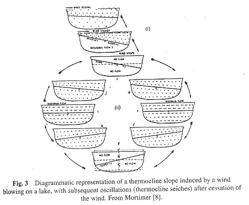
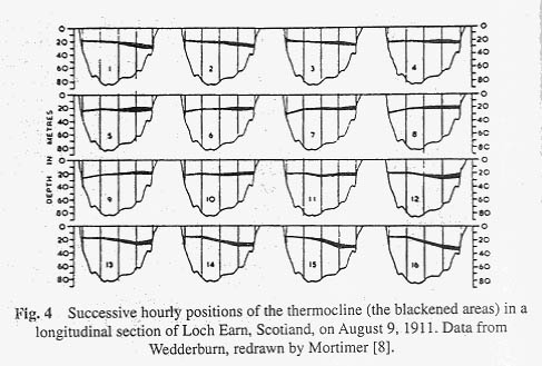
We have now come to realise that effective circulation is limited to the epilimnion during thermal stratification. We can amuse ourselves by letting a moderate wind blow on the lake. The surface water will be drawn to the leeward side inducing a moderate slope of (let us say) 1 millimetre per kilometre rising toward the leeward side. To maintain such a slope requires about 1000 times as much work as it would be to raise the level of the hypolimnion on the opposite side by the same distance. This work depends on the density difference between air and warm water on the one hand (density of water =1; density of air = 0.0012) and between warm and cold water on the other (density of water at 4 ° C = 1.00000; density of water at 20° = 0.99823). As a general rule then, we may expect a steep slope on the thermocline for a barely perceptible slope on the surface water. When the surface slope is 1 millimetre per kilometre, the thermocline slope (in the opposite direction) will be 1 meter per kilometre, and all this for quite a moderate wind. Let us suppose now that the wind ceases. The situation is unstable and the raised hypolimnion on the windward side pushes down and toward the leeward side, inducing a displacement of epilimnetic water from the leeward to the windward side of the lake. But due to the high momentum, the mark is overshot and a series of teeter-totter-like oscillations are set up, as shown diagrammatically in Figure 3, and for an actual set of observations from Loch Earn, Scotland, in Figure 4. The oscillations become damped (less violent) with time due to frictional resistance of the water itself. If a second wind is introduced, the oscillations may become further damped or forced depending on the relation of wind direction to that of thermocline slope.
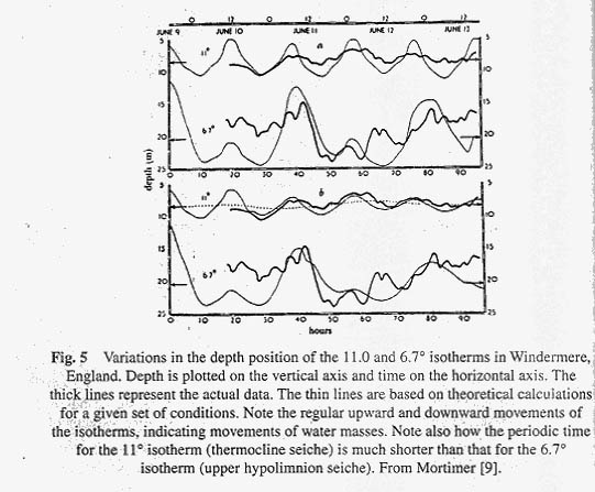
The oscillations that we have been discussing move about a node approximately in the centre of the lake, at a depth where thermal resistance is mixing at a maximum. The phenomenon is properly called a uninodal internal seiche. It is called internal because it occurs in the lake and is accompanied by little variation in the height of the lake surface. Uninodal seiches are the commonest and most easily measured of all internal seiches in lakes. Surface seiches are seldom observed except on the largest of lakes. They can be recognised by a periodic rise and fall of water level on a shore at one end of the lake. For uninodal internal seiches the vertical displacements of water are greatest at the windward and leeward ends, and least at the node. Horizontal displacements of water, on the other hand, are greatest at the node and least at the sides of the lake. One can verify this by dropping particles of dye into a swaying teacup. The best method for limnological measurement of internal seiches is to suspend a series of recording electrical thermometers at particular depths in the region of the thermocline (though anyone can record internal seiches using a water bottle and a hand thermometer as the only instruments). One can then chart the depth position of a particular temperature as it varies with time. Such a chart is shown in Figure 5 for the 11 ° isotherm from Windermere, an English lake. Note the periodic rhythm of the movements, which indicate the rise and fall of a particular water mass (with a temperature of 11 ° C). The movements of the 6.7 ° isotherm, also shown in Figure 5 differ from the 11 ° isotherm. Mortimer [8], from data of this sort, has concluded that there are two main types of internal seiches, the thermocline seiche moving about the interface between the epilimnion and the region of maximal density change in the thermocline, and an upper hypolimnion seiche moving about the interface between the lower thermocline and upper hypolimnion. The period of the upper hypolimnion seiche is generally longer than that of thermocline seiche. (The period is the time required for completing one cycle, or in general terms the time required transporting excess epilimnetic weight from one end of the lake to the other and backing again). For a small German lake, Lunzer Untersee (length 1.5 km) the period is but a few hours. For the larger Lake of Geneva (length 37-km) the period is increased to four days [9]. For even larger lakes the periods increase, and for the very largest lakes the effects of the rotating earth may become important in limiting the period.
The importance of understanding internal seiches cannot be overestimated. The disturbing influence of the internal seiche on attempts to measure the physical properties of lakes will be clear, and no less obvious will be De Moll's [10] observation that the microscopic plankton of the water mass in which it bathes. Even fishes and animal plankters (which can move to some extent independently of water movements) have their distribution partly determined by internal seiches. The seiche also appears to be particularly important in introducing turbulence into the hypolimnion, a region that would otherwise largely be stagnant. In short there is no aspect of limnology or freshwater biology that remains uninfluenced by the internal seiche.
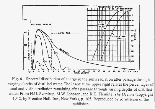
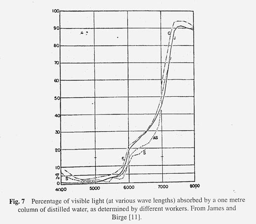
Before leaving the physical aspect of a lake we must briefly consider in more detail the absorption of the sun's radiation by lake water. The whole economy of the lake is dependent on the sun's energy because it is this energy that the microscopic plants (phytoplankton) and rooted aquatic vegetation use to make carbohydrates from CO 2 . We must first of all consider two factors: The nature of light incident on the lake surface, and the way in which water absorbs light of different wavelengths. There are three forms of light radiation of interest to us: visible light (wavelength 0.4-0.75 m ), ultraviolet light of shorter wavelength (<0.4 m ) and the infrared light of longer wavelength (>0.75 m ). Figure 6 shows the relative energy values for light of different wavelengths that is incident on the lake surface. Most of the light lies in the visible and infrared regions. The sun does emit ultraviolet radiation but the ozone layer in the earth's atmosphere effectively filters this out. Water absorbs light of different wavelengths in a characteristic way. The energy curves for the light not absorbed on passing through 0.1 – 100 meters of distilled water are also shown in Figure 6. Note that infrared light is almost completely absorbed by 1 meter of distilled water. When a plant physiologist wishes to study photosynthesis under high light intensity without overheating his plants he usually interposes a jar of water between the light bulb and the plant. Infrared radiation is a form of heat radiation and it is effectively filtered out of water. Visible light is absorbed by water to a much lesser extent. As the depth of water increases from 0.1 meters to 100 meters, note how the light becomes more and more effectively limited to a narrow band of blue light at a wavelength of about 0.5 m . That is the wavelength at which water absorbs the least amount of light, and it is for this reason that the water of clear deep lakes looks blue (sometimes the reflected blue of the sky is also involved). Although we could infer the absorption spectrum of distilled water from Figure 6, it is more clearly seen in Figure 7. The overall effect for sunlight passing through distilled water is that the light at any depth greater than a few meters is low in violet light (0.4 m ) because there is little of it incident on the surface of the lake and low in red and infrared light because the water has effectively absorbed it.
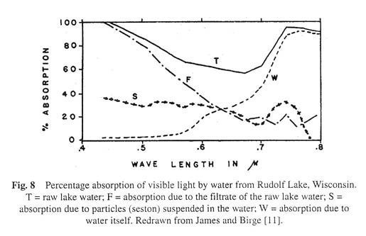
We have considered only distilled water up to now. Before turning to lake water we must recall another physical law: Beer's law which states that the percentage of incident light absorbed increases exponentially with the concentration of the light absorbing material. If the concentration is doubled the amount of light that is absorbed is more than doubled. Light absorbing materials present in lake water modify the picture so far presented. It is convenient to divide the light-absorbing matter into the particles (planktons plus debris) that can be removed by filtration, and those, which are soluble and pass through the filter. It has been found that the suspended particles of the plankton have a rather flat absorption curve, which shows slightly higher absorption at the lower visible wavelengths. These may be anomalies in the red end of the spectrum due to the absorption bands of chlorophyll. The soluble coloured materials consist mostly of humic substances derived from decaying vegetation. These impart a tea colour to the water. It is particularly strong in the waters of bog lakes. The colour may be so intense in some cases that the water appears almost black.
In simple terms we may think of the absorption of light by lake water as a tripartite function: light absorbed by water itself (curve W in Figure 8), light absorbed by the seston (curve S in Fig. 8) and light absorbed by the filtrate of lake water (curve F in Fig. 8). The curve T is the absorption curve for raw lake water. Analysis shows how it may be separated into three components.
I have attempted up to now to give a general picture of the absorption just after light has entered the water. Much of the light incident on the water is reflected. The amount of directional sunlight varies with the angle of the sun to the lake surface, and thus increases (2% to 40%) as the sun is displaced from the zenith, either during the day or season. Light may be reflected from clouds to the lake surface, and there are many other complicating factors out of place in a general discussion of this sort. So much for the physical background. With the backlog of information we are now in a position to look at the overall metabolism of the lake.
| Part II : Metabolism | up | previous | next | last |
Let us now look at the lake as an ecosystem, an open unit of space through which energy is flowing, and in which transformations of the energy are occurring. We are concerned mostly with organism-catalysed processes, and may accordingly neglect other forms of energy such as the potential energy of the lake with respect to a lower ocean.
Lacustrine organisms may be artificially divided into three groups on a spatial basis: the plankton (plant and animal) consisting of microscopic life in water; the nekton comprising larger, free swimming forms in the water (fishes etc); and the benthos, or bottom living organisms. We can speak of open water or limnetic community of organisms as distinct from littoral community associated with rooted plants in shallow water. Since we are concerned more with the metabolism of the lake, rather than a classification of its components, we shall largely bypass limnological terminology and consider trophic levels: the story of the eater and the eaten. These food relationships are shown in Figure 9.
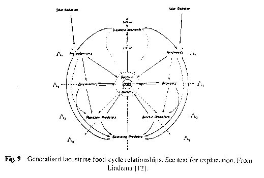
The trophic classification lies at the basis of all further discussion, so a few words of explanation may be appropriate. Let us designate the trophic levels as L-1, L-2, etc., and the energy content (measured by its calorific value) of a trophic level at a particular time as A-1, A-2, and so on. At the L-1 level ( º A 1 in Fig.9) are the producer organisms, which bring about a synthesis of organic matter directly from the absorbable energy of the sun's spectrum. These are the green phytoplankters, photosynthetic bacteria and rooted green plants. Feeding on the producers are herbivores of the L-2 level ( º A 2 in Fig.9), the zooplankters and the vegetation browsers. Also lying at this level are the heterotrophic bacteria and fungi, which may conveniently be termed as decomposers. They break down the organic matter of the dead organisms using part of the derived energy for the synthesis of new protoplasm and returning part to the water as nutrient for the further growth of the producers. At the L-3 level are carnivores, which feed on the herbivores of the L-2 level. We may exemplify the L-3 level by sunfish or predaceous diving beetles. Then of course there are larger carnivores (e.g., pike and bass) at the L-4 level which feed on carnivores at the L-3 level. In the sea an L-5 level is possible, but in lakes, mouths are more limited in size.
We must clearly distinguish among three commonly used measures of aquatic organisms: standing crop, removal rate and production rate. The first is the measure of the weight of organisms in a unit space at a particular time. Thus, the standing crop of algae on July 25 may have been 522,000 cells per litre of surface water. Removal rate is the yield. It is like the term harvest in agriculture or gallons of milk per day per cow, and involves the concept of weight removed in a given interval of time. Production is a concept involving turnover: it is the amount of organic matter synthesised under a unit area in unit time. It is meaningful to divide the production rate into a net rate, or the amount of weighable matter synthesised (under unit area in unit time) and a gross rate which takes into account the energy dissipated in making organic matter plus energy losses to higher members of the food chain. Suppose cabbages are grown on a plot of ground over a period of one year, the yield is the edible weight harvested. The total weight of plant material produced is the net production rate. In order to evaluate the gross production rate we must know the weight of cabbages eaten by rabbits and insects, and also the organic matter, which the plant synthesised but subsequently used for respiration. No process is 100% efficient. In order to live, the plant must oxidise part of the organic material, which it has already produced from sunlight and CO 2 .
One is often tempted to infer high production rates from high standing crops, but this is not always the case. The phytoplankton may be abundant in a lake and yet the turnover rates may be low. The converse is equally true. I was amused one summer at the University Biological Station when an unsuspecting person had removed our garbage pail. He claimed that it had been lying idle by the main garbage dump for weeks. In point of fact however, it was my practice to dump the garbage each morning and return the pail to our cottage every night. He had seen the pail in the same place; little realising how often it was moved and replaced. Removal and production rates may also be entirely two different things. A fisherman is tempted to say that the population of fish is low when he catches few, but the explanation may simply be that the fish has moved elsewhere. One must always be careful to think in terms of what has actually been measured.
Table-1 Production rates (net and gross) in G-cal cm -2 yr -1 and percent efficiencies for trophic levels of Cedar bog lake, Minnesota and Lake Mendota, Wisconsin. Data from Lindeman (1942)
Trophic Level |
Cedar Bog Lake Production rate |
Lake Mendota Production rate |
||||
Net |
Gross |
Efficiency |
Net |
Gross |
Efficiency |
|
L 0 |
£ 118,872 |
£ 118, 872 |
0.10% |
118,872 |
118,872 |
|
L 1 |
70.4 |
111.3 |
13.3 |
321 a |
480 a |
0.40% |
L 2 |
7.0 |
14.8 |
23.3 |
24 |
41.6 |
8.7 |
L 3 |
1.3 |
3.1 |
1 b |
2.3 b |
5.5 |
|
L 4 |
0.1 |
0.3 |
13.0 |
|||
a This figure is probably too high by 25%.
b This figure is probably too low as it does not include forage fish.
Although somewhat premature, it may be well to have a look now at the energy production rates (net and gross), which Lindeman [12] computed for the trophic levels of two lakes. These are given in Table 1. Two main principles will be noted: first, that production rates decrease exponentially with the trophic level; and secondly the efficiency with which one trophic level utilises the energy of the previous, increases with the trophic level. The first principle is more important to us for it focuses attention on green plants as the primary producers do. They convert the inedible energy of the sun into food material, which can be utilised by the plant, and saprophytic plant populations of the lake.
Coupled with the principles mentioned above, we may also note in passing, that the higher the trophic level, the more marked is the tendency for both the mass and the number of individuals to decline sharply. We quickly appreciate that microscopic algae outnumber bottom living animals, and these in turn the fish, but it is perhaps not so obvious that the same relations hold true for weight as well as number.
There is another point worth making at this time: the little things are the most active metabolically. Bacteria will reproduce a given weight in a few minutes; unicellular algae the same in a few hours; but mosquito takes days and a fish or a large rooted plant, months. As one passes from the large to small in the living world, the metabolic rate per gram of tissue rises exponentially as the weight of the individual decreases [13]. We may thus look to the microscopic algae (phytoplankton) of the lake as the most important producers, and bacteria as the most important decomposers.
From the metabolic point of view, the lake can be divided into two layers, an upper trophogenic zone in which photosynthesis predominates, and a lower trophogenic zone where decomposition is the rule. The line of demarcation is the compensation depth i.e., the depth at which the producers (L-1) respire energy as fast as they utilise it. The compensation depth is primarily determined by light penetration in the water. It may lie in the uppermost meter of water in a tea-coloured bog lake, or at depths of 17 meters and below in clear water lakes [14]. Although photosynthetic production is limited to the trophogenic zone, decomposition is by no means inactive there. Kleerekoper [15] has in fact suggested that the rate of organic matter decomposition in the epilimnion is many times greater than that in the hypolimnion, a principle perhaps to be expected because of the higher epilimnetic temperature.
While the benthos live in comparative comfort on the soft cushion of the mud, limnetic organisms are continually beset with the problem of sinking. Fishes and zooplankters can regulate their position in the lake to an extent dependent on the effectiveness of their swimming movements. With phytoplankters these movements are either ineffectual or lacking and in the absence of flotation factors they sink toward the depths of hell. The most important factor, particularly in the epilimnion, is the vertical turbulence of the water (induced by the wind) that keeps these small forms in suspension. We may consider other factors if we momentarily disregard turbulence and consider the velocity of fall of small bodies (less than 1 millimetre long) obeying Stokes' Law [16]. The rate of fall of these small forms varies directly with their excess density over the surrounding water, directly with the square of their “length”, but inversely with the viscosity of the medium (Stokes' Law) (The term excess density refers to the excess weight over and above a sample of water of equal volume). In other words, if viscosity and density difference are kept constant, a sphere of 1 millimetre diameter will sink 100 times more quickly than a sphere of one-tenth the diameter, ten thousand times more quickly than a sphere of one-hundredth the diameter, and a million times more quickly than a sphere the size of a small bacterial coccus (0.001 mm). Size is not only the important factor, for if the shape of an organism departs from that of a sphere, the sinking speed is lowered because of the increased frictional surface. External gelatinous sheaths, oil droplets, gas vacuoles and water storage are other mechanisms by which the sinking speed of an organism is reduced. This operates to reduce the excess density.
As a general rule we may expect all limnetic plankters except the largest to follow the pattern outlined by Stokes. In the thermocline and hypolimnion where vertical turbulence is reduced, the factors of form, density and viscosity become important in regulating the depth position. The rules that we have outlined above are probably not applicable to lake bacteria for they partly occur free in the water, and partly adsorbed on the surface of the plankters. This illustrates one of the many complicating issues not discussed.
We now have a fair, though abstract, picture of the plankton, to which we must add a few further points to complete the general scene. The rooted vegetation of the littoral region vies in importance with the phytoplankton as the main energy producer. This vegetation and even so the bottom sediment are richly coated with bacteria. The benthic animals of the mud live to a large extent on the partially decomposed plankton, and if they do not leave the lake basin (some as adult insects) they will in turn be decomposed by bacteria.
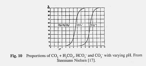
Within this framework let us now turn to the overall metabolism of the ecosystem. We can make a beginning, as did Mayow and Lavoisier for the living body, with the general aspects of gas exchange and energy in the lake. Recalling the perfect gas laws learned in elementary chemistry one can see how N 2 , though less soluble in water than oxygen, is actually present in greater amount – due to its higher partial pressure in the atmosphere. Remember also that gases become less soluble in water as the temperature is increased, each gas according to its own rules. But CO 2 (present in air only in minute amounts, 0.03% by volume) obeys an entirely different set of rules, because it enters into chemical combination with the water. Although the gas CO 2 may be put as such into an aqueous system, it will in part become hydrated (as H 2 CO 3 ) and changed into ionic forms (HCO 3 - and CO 3 + ) to an extent determined by the pH as shown in Fig. 10. In hard water lakes the dominant anion (negatively charged) is bicarbonate (HCO 3 - ) and it is balanced by cations (positively charged) of Ca ++ and Mg ++ . When the activities (concentrations) of Ca ++ and HCO 3 - ions exceed a certain value a precipitate of CaCO 3 is formed giving rise in some lakes to extensive deposits of marl. The point is if we are going to consider the respiration of a lake we must first appreciate the difference in chemical behaviour of the beginning and end products, O 2 and CO 2 .
Let us return now to our previous picture of trophogenic and tropholytic zones, corresponding roughly in summer to the epilimnion and hypolimnion. Due to the active photosynthesis (resulting in the production of O 2 ) and turbulence we may expect in the epilimnion, and in practice do find, that dissolved oxygen in epilimnetic water lies near the saturation point at all times. The situation is quite otherwise in the hypolimnion, for as we have seen (Part I) the thermocline barrier does not permit contact of hypolimnetic water with air. The penetration of dissolved materials into the hypolimnion is thus reduced to quite low values in summer. Since this is true (to a first approximation) the decomposition processes in the hypolimnion will be attended by a measurable decrease of O 2 and increase of CO 2 , as compared to the water in early spring. The severity of the depth decline of O 2 concentration in the hypolimnion depends on a number of factors, not the least of which are the form and the volume of the lake, as Thienemann [18] showed long ago. Suppose we have two lakes identical in surface area, with identical production rates and with the same penetration rates for dead particulate organic matter sinking down from the epilimnion; if one lake is much deeper than the other, the lake with the smaller volume of hypolimnetic water will be most rapidly depleted of oxygen. This is simply because the initial quantity of oxygen was small. Microbial breakdown of organic matter causes the oxygen depletion. Bacteria use O 2 and produce CO 2 during metabolism.
If we follow Hutchinson [19] and compute the aerial hypolimnetic O 2 deficit (the rate of oxygen consumption for a column of hypolimnetic water, unit area in cross section), then we can exclude the volume factor. This permits the limnologist to compare values for different lakes. If one accepts that the rate of oxygen consumption in the hypolimnion is proportional to the amount of particulate organic matter falling through to the hypolimnion, then at once we have a relative measure of the production rate. It is not a complete measure because not all of the organic matter synthesised sinks down to the hypolimnion. Part is broken down in the epilimnion and some pass to the outlet. Furthermore, not all of the particulate matter reaching the hypolimnion is decomposed. Much of it remains in the sediment. A further difficulty in this method is that a large part of the O 2 deficit is actually due to bacterial destruction of organic matter deposited in the mud.
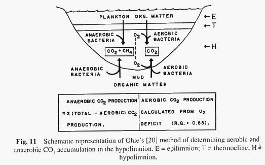
Ohle [20] has developed a subsidiary method (see Fig.11) based on the earlier work of Einsele. The basis of this method is that the CO 2 production in the hypolimnion is measured rather than O 2 depletion. There are two basically different types of bacterial metabolism, one, which proceeds in oxygenated environments (aerobic metabolism), and the other in oxygen poor environments (anaerobic metabolism). Using Ohle's method, one can calculate the CO 2 accumulated by aerobic processes from knowledge of O 2 consumed. The only assumption involved is that the respiratory quotient is 0.85, or in other words for every 100 O 2 molecules utilised, 85 molecules of CO 2 are produced (on the average). Empirical evidence leads us to believe that this is a reasonable assumption. Thus, we have accounted for part of the CO 2 accumulation as due to aerobic processes. The remainder must have arisen from anaerobic metabolism. However, it is (in general terms) true that only about half of the organic matter broken down by anaerobic processes ends up as CO 2 . The rest is liberated as methane (CH 4 ), also known as marsh gas. If we are to arrive at a value for the amount of organic matter broken down in the hypolimnion, we must add the weight of CO 2 produced aerobically, twice the CO 2 produced anaerobically. This value, when multiplied by a factor that converts the CO 2 produced to the organic matter (e.g., glucose) broken down, gives the total organic matter decomposed during the period of the study. The final step, before comparisons can be made among different lakes, is to refer the organic matter breakdown to a unit area of water. If we assume that the rate of organic matter breakdown is a relative measure of production rate, then we can compare the production rates of lakes, which lie in the same district: lakes which have roughly the same amount of sunlight energy falling on their surfaces.
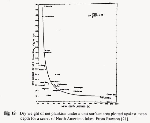
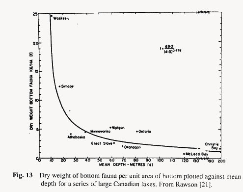
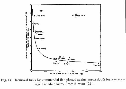
The interesting point is that the production rate rises as mean depth of the lake decreases. The shallower the lake (within limits) the higher is the production. The same is true (Rawson [21]) for standing crops of plankton and benthos, as well as for economic yields of fish (see Figs. 12, 13 and 14). As to why this should be is that with the smaller volume of lake water there is a more intimate contact of water with mud, and many of the nutrients needed for plankton growth are regenerated by decomposition processes in the mud.
So much for the beginning and end of metabolism. If we look in the middle, we find that the little that is known centres on inorganic chemicals, especially inorganic phosphorous and nitrogen compounds. The mean ionic composition of lake waters of the world [22] shows the dominant cations to be Ca++, Na+, Mg++ and K+ in that order. They are balanced to greater or lesser degree by HCO 3 -, SO 4 = and Cl- as the main anions in that order. These seven are the major ionic constituents. Lake water has quite a different chemical composition than seawater (where Na+ and Cl- are by far the most abundant ions). Of the less abundant inorganic constituents in lake waters only Si, Fe, Mn, N (NO 3 , NO 2 , NH 3 ) and P have been studied to any extent. They appear to be different because they may at times be present in concentration so low that they limit plant growth. The actual composition of any particular lake water will depend on the rate of supply of different ions from soil, rock and rain, the rate of removal by outlets and ion-exchange processes in lake sediments and the influence of organisms.
The nutritional requirements of any particular species of alga (the requirements vary greatly with the species) indicate what is needed for growth. If one compares the nutritional spectrum with the concentration of nutrients available in the water of a lake, some indication is had of those factors, which are most likely to limit continued growth. As a general rule phosphorous (as PO 4 º ) and nitrogen (as NO 3 - or NH 4 +) are most limiting in the aquatic environment, just as the farmer has found for the soil. But the story is indeed complicated for the limnologist to unravel. By way of example, phytoplankters can store excess phosphorous under certain conditions, and be temporarily capable of good growth in cultures deprived of that element [23]. In nature, it may be the phosphate concentration which occurred a week before an algal bloom that was the important factor – not the phosphate concentration at the time the bloom began.
It is important to realise that chemical analyses of the lake ecosystem mean little in terms of metabolism unless one understands the importance of the chemicals to the organisms inhabiting the lake. The physiological meaning of chemical studies in the field rests rather strongly on information obtained in the laboratory. The reverse may also be true. Rodhe [23] reported the presence of an organic factor in lake water, which markedly lowered the phosphate requirements of the diatom Asterionella formosa . A chemical knowledge of this factor could aid considerably in physiological work.
It would not be proper to leave the study of lake metabolism without mentioning the profound influence of dissolved oxygen on chemical transformations in the hypolimnion. Since this involves an understanding of oxidation-reduction processes we must diverge briefly to introduce the concept of oxidation potential.
A substance undergoing oxidation loses electrons. This is the most precise definition of oxidation. Thus, reduced ferrous iron is oxidised to the ferric state:
Fe ++ = Fe +++ + e -
A migration of electrons is involved in any oxidation-reduction reaction. The electrical work done in transporting electrons to an electrode can be measured by immersing an unattackable electrode in the system. If the system is thermodynamically reversible, the electromotive force set up at the electrode is given as:
E h = E 0 + k log (oxidised products) / (reduced reactants)
E 0 is the standard potential for the system with reference to the potential set up at a standard cell under defined conditions (one of which is a pH of 0). The constant k is of little concern to us here. The terms in parentheses refer to the concentrations (activities) of the reactants and products. The point of significance is that the oxidation potential, in absence of any variation in temperature and pH, is a measure of the ratio of oxidised to reduced members in a particular reaction. When the concentration (activities) of the reactants and products are equal, then the logarithmic term on the right disappears (log 1= 0) and E h = E 0 . The value in E 0 in volts has a different value for different systems.
There are various reasons why the theoretical treatment of oxidation-reduction cannot be directly applied to ecological systems, but in temporarily bypassing these difficulties, Mortimer [24] has provided great insight into otherwise perplexing data. The oxidation potential in a lake is primarily regulated by the content of dissolved oxygen in the water. The oxidation potential of aerated surface water at pH 7 lies around 0.5 volts. This potential does not markedly decline until the oxygen concentration falls from 10 to 2 mg per litre or less. For lake systems the following “limnological E 0 ” (at pH 7) values are of interest:
NO 3 - to NO 2 -………………..0.45-0.40 volts
NO 2 to NH 3 …………..…… 0.40 – 0.35 volts
Fe +++ to Fe ++ ………………....0.30 – 0.20 volts
SO 4 = to S=……………….….0.10 to 0.06 volts
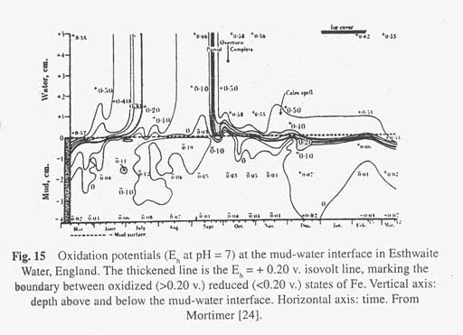
Oxygen in the hypolimnion is first depleted in water that is in contact with mud. This happens only when the water of hypolimnion has been out of contact with air for several weeks (in some cases the isolation may be due to an ice cover on the lake as well as to the mixing barrier of the thermocline, for either one prevents a mixture of air with water). Oxidation potentials at the mud-water interface at 14 meters depth throughout the year are shown in Figure 15 for Esthwaite Water, England. These potentials are all referred to a pH of 7 (so as to make them comparable). The disappearance of the E 7 (E h at pH 7) = 0.2 v isovolt line from the mud during summer stratification indicates the time at which the mud surface becomes sufficiently reducing to convert most of the ferric iron into ferrous state (at a potential of 0.20 volts most of the iron is in the ferrous state). This is a change that can be visually observed. The original oxidised surface was coloured brown due to the presence of ferric hydroxide. As the ferric iron changes to ferrous the surface mud blackens, just as does the red rust of iron when it is chemically reduced. The slow, approximately molecular diffusion of the 0.20 isovolt line in the mud may be compared with its rapid turbulent diffusion in the overlying water of the hypolimnion (see Fig. 15). Note also how the 0.20 isovolt line nearly reached the surface of the mud in February under the protection of an ice cover on the lake. The method of presenting data that is used in Figure 15 is a little difficult to get used to, but to the limnologist it is the only way of showing the three variables of concentration, depth and time on a sheet of paper. The data are for samples of mud and water at a particular site throughout the year.
The conversions of iron are not the only processes that accompany low oxidation potentials in deep water. The conversion of ferric to ferrous iron is preceded by the conversion of nitrate to ammonia through brief intermediate stages of nitrite and hydroxylamine (NH 2 OH). As the potential is lowered further sulphide is formed from sulphate, and the deep water begins to smell of H 2 S, a gas commonly associated with the odour of rotten eggs. Coloured materials of unknown nature pass from the mud to darken the overlying water.
When the thermocline breaks down in the fall, there is no longer a mixing barrier, which isolates the hypolimnion from aerated water (see Fig. 15). Oxygenated water from above mixes with the reduced water of the hypolimnion. The substances liberated by the mud are oxidised and precipitated. Iron first precipitates as the insoluble ferric phosphate, and later when all the phosphate has been used up, as ferric hydroxide. These precipitates tend to sink back to the mud, though part may be utilised for plant growth before sinking is complete. Other liberated products not so strongly affected by conditions of pH and E h may be transported to other parts of the lake, but the sediment acts as a trap for iron and phosphorous. It is unfortunate to leave this brief presentation without introducing the perspective of time, but I shall have to leave that intellectual exercise to your imagination. What happens as an orginally deep lake basin is filled in with sinking plankton and mineral matter from the surrounding land? An application of the principles already presented permits at least a partial answer.
| An apology to the biologist | up | previous | next | last |
In the time allotted I have discussed those properties, which I feel are basic to the understanding of the lake as a whole. To assume as I have that trophic levels are homogenous has led to my neglect of the many remarkable phenomena, which attract the limnologist to his discipline. Apologies.
| Surprises for the future | up | previous | next | last |
It is difficult to predict what the important future developments in limnology will be, except the most important are probably unknown to us at the present time. However, on the basis of past research it seems that there are four areas, which could repay critical study:
• The development of quantitative techniques and theory of the study of turbulent transfer processes in the lake and between the lake and its surroundings. It is remarkable that our meagre knowledge of the currents in the hypolimnion has mostly been inferred by indirect means, and the factors influencing the heat budget of a lake cannot be adequately measured.
• An understanding of the dynamics of phytoplankton growth on a molecular level. Lefevre and his collaborator [25] have recently amassed data to show that antibiotics may be of great importance in regulating phytoplankton production and succession.
• A limnological application of Riley's [26] quantitative approach to the dynamics of marine plankton.
• Extension and development of absolute dating methods as applied to lake sediments. If absolute time scales are available, then quantitative estimates of the sediment deposition rates might have quantitative measures of production rates during past time. These could then be related to other factors such as changing climate.
| References and Notes | up | previous | next | last |
| Address: | up | previous |