Issues: 1 2 3 4 5 6 7 8 9 10 11 12 13 14 15 16 17 18 19 20 21 22 23 24 25 26 27 28 29 30 31 32 33 34 35 36 37 38 39 40 41 42 43 44 45 46 47 48 49 50 51 52 53 54 55 56 57 58 59 60 61 62 63 64 65 66 67 68
BharathSetturu1, Vinay S1Ramachandra, T V* 3. Materials & Method 3.1. Study AreaKodagu (Coorg) district in Karnataka is also known as “Kashmir of south” and “Switzerland of India” surrounded by Hassan district in the north, Mysore district in the east, Dakshina Kannada on the west and Kerala State to the south (Figure 1) with an area of 4,102 km2 (2.4% of Karnataka’s geographical area) having population of 5,54,762 as per 2011 census. The population density shows 135 persons per sq.km. The elevation ranges from 900 to 1750 m above mean sea level and mean temperature range from 20°-24°C in with an average rainfall of 4000 mm. Madikeri, a hill town is the head quarter and located 252 km away from Bengaluru (Karnataka’s capital).The region is home to endangered Myristica swamps having Critically Endangered Syzigiumtravancoricumand Gymnacrantheracanarica(Vulnerable) are amongst many other species. Realizing the rates of degradation Union government has proposed to protect natural ecosystems by considering as conservation units such as protected areas (PA) and district has 3 WLS namely Pushpagiri, Talacauvery, Bramhagiri and one NP i.e. Nagarahole. 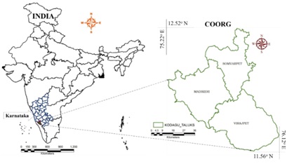 3.2. MethodFigure 2 outlines the overall method adopted for the analysis. The process of land use classification, modelling likely changes and identifying ecological fragile zones are carried out in five phases i) Classification (ii) Modelling (iii) Computing weightage metric score for prioritisation. 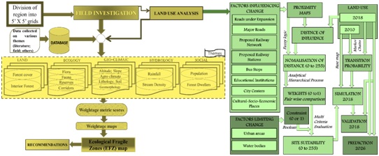 (a) generation of False Color Composite (FCC) of remote sensing data (bands–green, red and NIR), (b) selection of training polygons by covering 15% of the study area (polygons are uniformly distributed over the entire study area) (c) loading these training polygons co-ordinates into pre-calibrated GPS, collection of the corresponding attribute data (land use types) for these polygons from the field, (d) supplementing this information with Google Earth and (e) 60% of the training data has been used for classification, while the balance is used for validation or accuracy assessment. The land use analysis was done using supervised classification technique based on Gaussian maximum likelihood algorithm with training data. GRASS GIS (Geographical Resources Analysis Support System, http://ces.iisc.ac.in/grass) a free and open source software with the robust support for processing both vector and raster data has been used for analyzing RS data. (ii) Modelling and visualization: Likely land uses in 2026 is generated considering (1) Markov Chain transition of base land uses, (2) evaluating the driving factors and constraints, (3) weightage metric score by fuzzy AHP based estimation and site suitability maps generation by MCE, (4) simulation and future prediction of land use by MC-CA algorithms. Land use maps of 2010, 2018 were evaluated by MC analysis to compute the transition probability. The driving forces of land use changes and constraints were identified based on the land use history, review of literature and policy reports. Major drivers of landscape transitions are slopes, major highways, industries, core residential areas. Constraints perceived are water bodies, river coarse, protected areas and reserve forest. The contributing factors for different land uses were normalized between 0 and 255 through fuzzification- 255 indicates maximum probability of change, while 0 indicates of no changes (Figure 3). The pair wise comparison matrices were generated across three agro climatic regions and their relative weights as Eigen vectors were estimated using AHP (Bernasconi et al., 2010) to measure the degree of importance between criteria or factors i and j. A response matrix A= [aij] is generated to measure the relative dominance of item i over item j. A is constructed with the decision maker’s assessments aij, as pairwise comparisons that follow a uniform probability distribution. Validation was carried out based on the simulated land use, comparing the simulated land use map as against the actual land use map using Kappa Statistics. Model was calibrated by varying the input variables in order to achieve higher accuracy. Calibrated model was used to predict and visualize the land use change pattern for the year 2026. 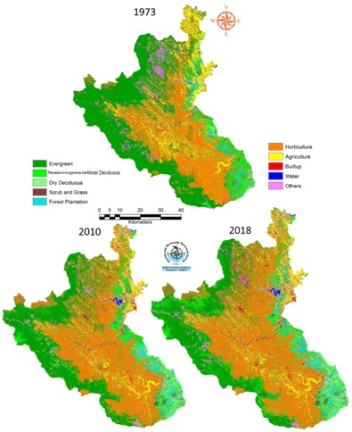  ..............(1) ..............(1)
|