3.    MATERIALS AND METHODS

3.1 Study area
The Uttara Kannada of Karnataka State, where the study area Kathalekan has been chosen (Fig.3.1), forms the northern end of the central Western Ghats and is ecologically and biogeographically important as the northern most limit of the distribution of major evergreen forest formations and many evergreen endemic tree species (Devar, 2008). The total forest cover of the district is 7,807 sq.km out of total geographic area of 10,291 sq.km. (Bhattacharya and Gadgil, 1993); the district has the highest forest cover in Karnataka. Recent vegetation analysis in Uttara Kannada district by Ramachandra and Savitha (2007) shows that 4325 sq.km under evergreen, 843 sq.km under deciduous, 580 sq.km. under scrub savanna and grasslands and 599 sq.km under barren or waste land categories, highlighting the large scale changes in land cover (http://wgbis.ces.iisc.ernet.in/energy/water/paper/ETR24/index.htm).

‘Kathalekan’ is the name of a hamlet in the Malemane village of Siddapur taluk towards the south-east of Uttara Kannada. It is situated between 14^o 26’ N to 14^o 27’N  and 74^o 73’  E to 74^o 75’ E. Kathalekan, which has just three families living in it,  probably had more population once upon a time, when the adjoining hills and some parts within it were under shifting cultivation. Today the hamlet is a largely forested area without any means to trace its geographic boundaries. Therefore for this study was chosen a total area of 2.25 km² (in a square shape of 1500m x 1500m). The forest is administered by the Siddapur Range of Sirsi Forest Division in the Canara Circle.

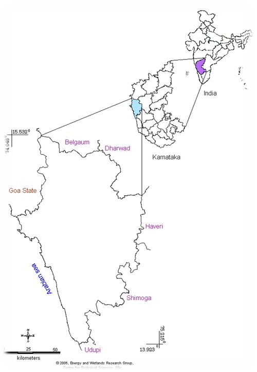
Figure  3.1: Study area – Kathalekan, Uttara Kannada district, Karnataka State, India

3.2 Topography and Climate

In Uttara Kannada district the Western Ghats are low not exceeding 600 to 700 m in most places. Kathalekan has altitude ranging from 500 to 700 m. It is surrounded on all sides by hill ranges and towards its south is steep gorge through which flows the river Sharavathi. The terrain within it is also very uneven with valleys and hills. Some of the valleys are endowed with perennial streams having swamps alongside them. Generally it has a tropical, humid climate. The climate does not show marked variation in both seasonal and diurnal temperature. The hottest months of the year are March, April, and May and the coldest months are December, January and February. Kathalekan receives good rainfall as the annual rainfall measured in the adjoining Mavingundi is 3435 mm. The bulk of the rainfall is from the south-west monsoon between June and October. The mean monthly rainfall during this period is: June: 813 mm; July: 1197 mm; August: 982 mm; September: 206 mm; 115 mm. January and February are practically rainless months whereas remaining months have rainfall less than 100 mm.  Pre-monsoon summer showers are received during April-May.

3.3 Selection of study area and devising sampling methods

Preliminary reconnaissance study of the region was conducted in January 2009 by trekking over the entire study area and familiarizing with the terrain that consists of hills and valleys, streams and swamps, evergreen forests, savanna grasslands and rocky places and very limited agricultural areas. Topographic maps of the Survey of India (1: 50,000 scale) and Google imagery were used during the preliminary field surveys.

It was then decided to select a study area of 1500 m x 1500 m considering the time and effort involved. The area has been further divided into nine grids each of 500 m² for detailed flora investigation. Figure 3.2 illustrates the study area as per Google images (http://www.googleearth.com). It was decided to sample the vegetation in each grid by using transect cum quadrat method (Sameer Ali et al., 2007). A transect of 180 m length and Quadrats of 20×20 m area were laid along the transect, alternately on either side of the transect for trees (Figure 3.3); sub-quadrats were laid within the tree quadrats for study of shrub layer and herb layer. An inter-quadrat distance of 20 m was maintained between the tree quadrats. Species-area relationship was worked out to appropriate number of sampling units - quadrats for trees, shrubs and herbs.

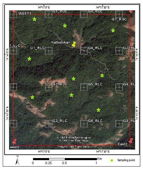
Figure 3.2: Study grids in Kathalekan as per Google image (http://www.googleearth.com)

3.3.1 Sampling of Trees:  In each quadrat of 20 m×20 m all the trees having girth ≥ 30 cm above the ground were enumerated. The girth at breast height (GBH) of every tree was measured in cm using a measuring tape, and approximate height recorded in m. The climbers and epiphytes associated with the trees were noted.

3.3.2 Sampling of Ground vegetation: The ground layer of shrubs (+1 m height but with GBH < 30 cm) were sampled using two sub quadrats of 5×5 m each, located within the tree quadrat, as shown in Figure 3.3. Tree saplings and shrubs as well as tall herbs were enumerated in these shrub quadrats.

Within the 5×5 m sub quadrats, two quadrats of one square meter each were placed diagonally as shown in Figure 3.3, for sampling the diversity of herb layer (plant less than 1 m height). The herb layer included herbs, tree seedlings as well as well as young ones of climbers and lianas. Due to practical constraints of time, repeated sampling to enumerate the seasonal herbs was not possible.

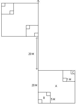
Figure 3.3: Transect with quadrats for sampling vegetation:  A-Trees, B- Shrubs, C- Herbs

3.4 Description of the study localities: The following general details were recorded in field data book from each sampled locality.

1. Location: Grid no and any local name existing for the Grid.
2. Patch type: Evergreen, semi evergreen, moist deciduous, scrub, savanna etc
3. Transect number
4. Nature of terrain: Steep slope/ Moderate/ Low to flat/Undulating
5. Rock outcrops, or rockiness: High// Moderate/ Poor to nil
6. Nature of rock: Lateritic /Non-lateritic
7. The occurrence of stream associated with the site
8. Soil erosion on the site: High/ Moderate/ Least
9. Nearest human habitation (distance)
10. Notes on human interference viz., lopping, tree cutting, burning, fuel extraction, litter collection, cattle grazing and any other activities
11. Sacred value
12. Non-Timber Forest Produce (NTFP) collection

3.5 Collection of Secondary Data: The ecological history of the region was compiled from published literature and books as well as based on interviews with the local people.  The study by Chandran (1993, 1997) constitutes the basic reference literature for this work. Some historical data was gathered from the previous study conducted in the area, as well as from field observations (such as old roads, timber-skidding areas, savanna-grasslands used earlier as shifting cultivation sites, patterns of forest succession etc.)

3.6 Mapping: An aerial imagery of the study area was downloaded from Google images website (http://www.googleearth.com). The relevant topo-maps available at the Energy and Wetlands Research Group (EWRG), Centre for Ecological Sciences (CES), Indian Institute of Science (IISc) field Station at Kumta taluk, Uttara Kannada district, Karnataka 581343, were referred to. Latitudes and longitudes of the sampling points at field were noted with the help of Global Positioning System (GPS). These points were plotted in the map with the help of GIS (Geographic Information System) software - MapInfo (7.5 version).

3.7 Ecological Measurements: Various ecological indices were computed to understand the diversity, relative abundance and dominance of species (Sameer Ali, et al. 2007). Indices include:

3.7.1. Species diversity (Shannon-Weiner Diversity Index): Diversity is an indicator of status of an ecosystem. It consists of two components, the variety and the relative abundance of species. The higher value indicates higher diversity. Diversity of trees and shrubs were estimated using the Shannon Weiner’s method. (Ludwig and Reynolds, 1988).The value ranges between 1.5 and 3.5 and rarely surpasses 4.5. Shannon Weiner’s index of diversity is calculated by the formula

    H’   = Σ [(n_i/N) ln (n_i/N)]

Where,  H’ = Shannon’s diversity index,   n_i = Number of individuals belonging to the ‘i’ species,   N = Total number of individuals in the sample.

3.7.2 Species dominance (Simpson’s Index): The species dominance is estimated by using Simpson’s index of dominance. It is suggested that the diversity was inversely related to the probability that two individual picked up at random belong to the same species. (Krebs, 1988)

Simpson’s Dominance,     D = Σ (P_i) ²
Where   P_i   = Proportion of species ‘i’ in the community

3.7.3 Species evenness Index (Pielou, 1996): Evenness index give an idea about the evenness in the species distribution. E approach to ‘0’ as single species become more dominant and this value increases when species become more evenly distributed. It is calculated by.

    E = H’/ ln(S)
Where, H’ = Shannon’s index,   S = Species richness (Total number of species)

3.7.4 Other parameters  (Sameer Ali, et al., 2007)

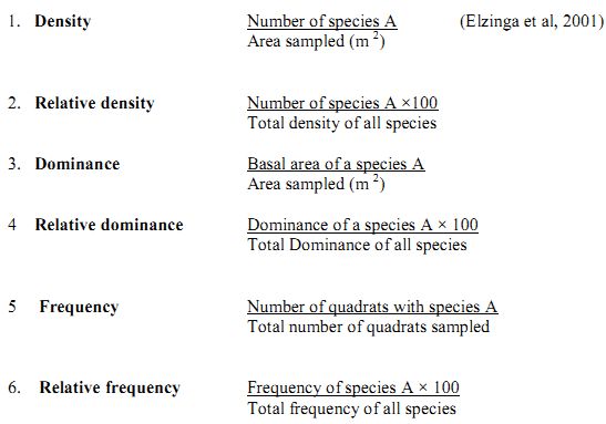
3.7.5 Importance Value Index (IVI): Importance Value Index is a significant parameter in any ecological assessment. It is an indicator of ecological success of the species. IVI was calculated according to Curtis and Macintosh (1951) and the formula is given below.

                        IVI =   Relative density + Relative dominance + Relative frequency.