NAME

KEYWORDS

SYNOPSIS

DESCRIPTION

Since a new raster map is created during the binning, the binning of points depends on the current computational region settings (extent and resolution) by default (see more about binning below). When using the -e flag, the binning will be done in the extent of the point cloud, so the resulting raster will have extent based on the input point cloud. When the resolution=value parameter is used, the binning is done using the provided resolution and the resulting raster will have that resolution (see more below for more information about extent and resolution management).

r.in.lidar is designed for processing massive point cloud datasets, for example raw LiDAR or sidescan sonar swath data. It has been tested with large datasets (see below for memory management notes).

Binning

In the basic case, binning is a method which counts the number of points which fall into one raster cell, i.e. bin. The number of points per cell (bin) indicates the density of points in the point cloud. The cell (bin) is always square or rectangular in case of r.in.lidar because the result is GRASS GIS 2D raster. The result of binning where the number of point per cell is counted is sometimes called 2D (two dimensional) histogram because a histogram is used in univariate statistics (in one dimension) to count the number samples falling into a given bin.

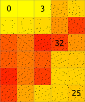
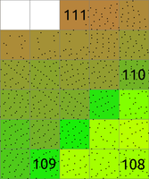
Figure: The binning on left was used to count number of points per (sometimes also called 2D histogram). The numbers in cells are examples of counts, the rest is represented by the color. The binning on right was used with mean to create a surface based on the values associated with the points. The numbers show examples of cell values. Note also the cells without any points which were assigned the NULL value.

Statistics

n

This computes the number (count) of points per cell. The result is a indicator of spatially variable density of points in the given area.

min

This finds the minimum of point values in each cell. It can be useful when finding topography in a forested or urban environment and there is a lot of points per one cells (terrain is oversampled considering the desired resolution). It can also create surfaces independent on the noise from premature hits as it will always select the lowest point.

max

This finds the maximum of point values in each cell. In connection with base_raster it can yield maximum vegetation of feature height per cell. For this purpose, it is usually much more appropriate than mean which would yield heights mostly influenced by the vertical distribution of points.

range

This computes the range of point values in each cell. The range of Z coordinates per cell can be used as a rough estimate of vegetation height when the cells are small enough, slopes low and the area is mostly vegetated. However, for more profound analysis, the base raster together with different statistics is recommended.

sum

This computes the sum of point values per cell. This is useful especially when intensity is used as a value (flags -i and -j).

mean

This is a mean (average) value of point values in cell. When used with Z coordinates (the default) and points from the ground class, the resulting raster is a digital elevation model. When intensity is used as a point value, the resulting raster contains mean intensity per cell. Note that mean gives heights influenced by the vertical distribution of points

stddev

This computes the standard deviation of point values for each cell.

variance

This computes the variance of point values for each cell. Variance and derivatives use the biased estimator (n) [note that this might be subject to change].

coeff_var

This computes the coefficient of variance of point values for each cell. Coefficient of variance is given in percentage and defined as (stddev/mean)*100.

median

This computes the median of point values for each cell

percentile

p^th (nth) percentile of points in cell

skewness

This is a skewness of point values in cell

trimmean

This is a trimmed mean of point values in cell. Trimmed mean also know as truncated mean is a mean computed after discarding values at the low end and at the high end. How many values to discard is given by the trim option in percent. In statistics the usual percentage of trimmed values ranges from 5 to 25 percent.

Filtering

g.region s=s-0.000001

The zrange parameter may be used for filtering the input data by vertical extent. Example uses include filtering out extreme outliers and outliers on relatively flat terrain. This parameter can be also used for cutting the point cloud into vertical sections preparing it for further processing by separate sections, together as if it would be an imagery group (see i.group), or combined into a 3D raster using r.to.rast3. In for these last examples, it might actually be more advantageous to use r3.in.lidar module. The zrange parameter is especially powerful when used together with the base_raster parameter. The zrange is applied to Z values after the base_raster reduction.

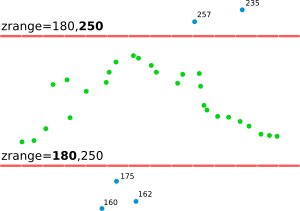
Figure: This is the principle of zrange filter. Points with the Z coordinate value below the lower value in the range (here 180) are filtered out (blue points) and same applies for points above higher value in the range (here 250). All other points are preserved (green points).

A LiDAR pulse can have multiple returns. The first return values can be used to obtain a digital surface model (DSM) where e.g. canopy cover is represented. The last return values can be used to obtain a digital terrain model (DTM) where e.g. the forest floor instead of canopy cover is represented. The return_filter option allows selecting one of first, mid, or last returns. Return number and number of returns in the pulse associated with each point are compared to determine if the point is first, mid, or last return.

LiDAR points often come as already classified into standardized classes. For example, class number 2 represents ground. For other classes see LAS format specification in references. The class_filter option allows selecting one or more classes using numbers (integers) separated by comma.

In varied terrain the user may find that min maps make for a good noise filter as most LIDAR noise is from premature hits. The min map may also be useful to find the underlying topography in a forested or urban environment if the cells are oversampled.

The user can use a combination of r.in.lidar output maps to create custom raster-based filters, for examplee, use r.mapcalc to create a mean-(2*stddev) map. (In this example the user may want to include a lower bound filter in r.mapcalc to remove highly variable points (small n) or run r.neighbors to smooth the stddev map before further use.)

Note that proper filtering of the input points in not only critical for the analysis itself but it can also speed up the processing.

Reduction to a base raster

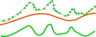
Figure: This is a profile of base raster (in orange) representing digital elevation model and selected points, e.g. first return, from point cloud (green dots). By default the points would create a digital surface model (thin brown line) but after reducing the Z coordinates using the base raster, the created surface is a derived from the height of points relative to the base raster.

Setting extent and resolution

Since the creation of raster maps depends on the computational region settings (extent and resolution), as default the current region extents and resolution are used for the import. When using the -e flag along with the resolution=value parameter, the region used for the new raster will be based the point cloud extent and the provided resolution. It is therefore recommended to first use the -s flag to get the extents of the LiDAR point cloud to be imported, then adjust the current region extent and resolution accordingly, and only then proceed with the actual import. Another option is to automatically set the region extents based on the LAS dataset itself (-e flag) along with the desired raster resolution. The best option is to know the point cloud extent ahead, e.g. from tiling scheme, and use it. See below for details.

Since the r.in.lidar generates a raster map through binning from the original LiDAR points, the target computational region extent and resolution have to be determined. A typical workflow would involve the examination of the LAS data's associated documentation or the scan of the LAS data file with r.in.lidar's -s (or -g) flag to find the input data's bounds.

Another option is to automatically set the region extents based on the LAS dataset extent (-e flag) along with the desired raster resolution using the resolution parameter.

Using the -s scan flag, the extent of the input data (and thus point density) is printed. To check this is recommended before performing the full import. The -g shell style flag prints the extent suitable as command line parameters for g.region.

A simpler option is to automatically set the region extents based on the LAS dataset (-e flag) along with the target raster resolution using the resolution parameter. Also here it is recommended to verify and optimize the resulting region settings with g.region prior to importing the dataset.

NOTES

Format and projection support

LAS file import preparations

Also note that the scanning does not apply any filters, so the extent determined by scanning can be theoretically bigger than the extent actively used during the binning. This behavior ensures that the newly created raster has always the same extent regardless the filters used. However, for most cases (considering the point cloud and the resolution used) there is no difference between the extent without filters applied and the extent if the filters would be applied.

Memory consumption

While the input file can be arbitrarily large, r.in.lidar will use a large amount of system memory (RAM) for large raster regions (> 10000x10000 pixels). If the module refuses to start complaining that there isn't enough memory, use the percent parameter to run the module in several passes. In addition using a less precise map format (CELL [integer] or FCELL [floating point]) will use less memory than a DCELL [double precision floating point] output map. For method=n, the CELL format is used automatically.

The mean and range methods will use average amount of memory (comparing to other methods). Methods such as n, min, max, and sum will use less memory, while stddev, variance, and coeff_var will use more.

The memory usage for regular statistics mentioned above is based solely on region (raster) size. However, the aggregate functions median, percentile, skewness and trimmean will use more memory and may not be appropriate for use with arbitrarily large input files without a small value for the percent option because unlike the other statistics memory use for these also depends on the number of data points.

The default map type=FCELL is intended as compromise between preserving data precision and limiting system resource consumption.

Trim option

Trim option value is used only when calculating trimmed mean values. Attempt to use it with other statistical methods will result in an error.

EXAMPLES

# set the computational region automatically, resol. for binning is 5m
r.in.lidar -e -o input=points.las resolution=5 output=lidar_dem_mean
g.region raster=lidar_dem_mean -p
r.univar lidar_dem_mean

Finding suitable extent and resolution

A simpler option is to automatically set the region extents based on the LAS dataset (-e flag) along with the target raster resolution using the resolution parameter. Also here it is recommended to verify and optimize the resulting region settings with g.region prior to importing the dataset.

For the output raster map, a suitable resolution can be found by dividing the number of input points by the area covered (this requires an iterative approach as outlined here):

# print LAS metadata (Number of Points)
r.in.lidar -p input=points.las
#   Number of Point Records: 1287775

# scan for LAS points cloud extent
r.in.lidar -sg input=points.las output=dummy -o
# n=2193507.740000 s=2190053.450000 e=6070237.920000 w=6066629.860000 b=-3.600000 t=906.000000

# set computation region to this extent
g.region n=2193507.740000 s=2190053.450000 e=6070237.920000 w=6066629.860000 -p

# print resulting extent
g.region -p
#  rows:       3454
#  cols:       3608

# points_per_cell = n_points / (rows * cols)
# Here: 1287775 / (3454 * 3608) = 0.1033359 LiDAR points/raster cell
# As this is too low, we need to select a lower raster resolution

g.region res=5 -ap
#  rows:       692
#  cols:       723
#  Now: 1287775 / (692 * 723) = 2.573923 LiDAR points/raster cell

# import as mean
r.in.lidar input=points.las output=lidar_dem_mean method=mean -o

# import as max
r.in.lidar input=points.las output=lidar_dem_max method=max -o

# import as p'th percentile of the values
r.in.lidar input=points.las output=lidar_dem_percentile_95 \
           method=percentile pth=95 -o

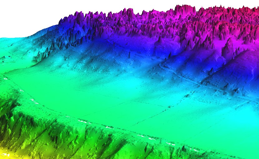
Mean value DEM in perspective view, imported from LAS file

Further hints: how to calculate number of LiDAR points/square meter:

g.region -e
  # Metric location:
  # points_per_sq_m = n_points / (ns_extent * ew_extent)

  # Lat/Lon location:
  # points_per_sq_m = n_points / (ns_extent * ew_extent*cos(lat) * (1852*60)^2)

Serpent Mound dataset

The sample LAS data are in the file "Serpent Mound Model LAS Data.las", available at appliedimagery.com:

# print LAS file info
r.in.lidar -p input="Serpent Mound Model LAS Data.las"

# using v.in.lidar to create a new location
# create location with projection information of the LAS data
v.in.lidar -i input="Serpent Mound Model LAS Data.las" location=Serpent_Mound

# quit and restart GRASS in the newly created location "Serpent_Mound"

# scan the extents of the LAS data
r.in.lidar -sg input="Serpent Mound Model LAS Data.las"

# set the region to the extents of the LAS data, align to resolution
g.region n=4323641.57 s=4320942.61 w=289020.90 e=290106.02 res=1 -ap

# import as raster DEM
r.in.lidar input="Serpent Mound Model LAS Data.las" \
           output=Serpent_Mound_Model_LAS_Data method=mean

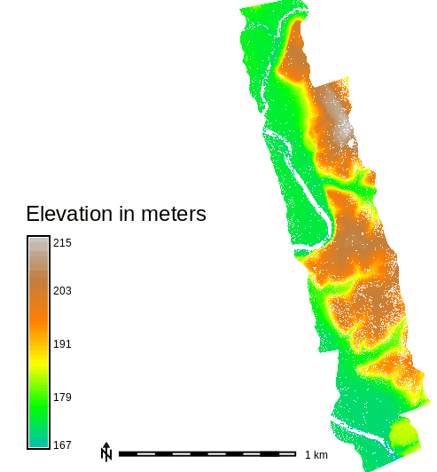
Figure: Elevation for the whole area of Serpent Mound dataset

Height above ground

g.region raster=elevation -p
r.in.lidar input=points.las output=mean_height_above_ground base_raster=elevation method=mean

Multiple file input

points1.laz
points2.laz
points3.laz

/home/user/data/points1.laz
/home/user/data/points2.laz
/home/user/data/points3.laz

ls /home/user/data/*.laz > /home/user/data/filelist.txt

dir /b c:\users\user\data\*.laz > c:\users\user\data\filelist.txt

g.region raster=elevation -p
r.in.lidar file=/home/user/data/filelist.txt output=mean_height_above_ground base_raster=elevation method=mean

import glob
import grass.script as gs
    
file_list_name = '/home/user/data/filelist.txt'
with open(, mode='w') as file_list:
    for path in glob.iglob('/home/user/data/lidar/*.las'):
        file_list.write(path + "\n")

gs.run_command('r.in.lidar', file=file_list_name,
               output='mean_height_above_ground',
               base_raster='elevation' method='mean')

KNOWN ISSUES

• The "nan" value (as defined in C language) can leak into coeff_var raster maps. Cause is unknown. Possible work-around is: r.null setnull=nan or r.mapcalc 'no_nan = if(map == map, map, null())'.
• Only one method can be applied for a single run and multiple map output from a single run (e.g. method=string[,string,...] output=name[,name,...] or n=string mean=string) is no supported.

SEE ALSO

REFERENCES

• V. Petras, A. Petrasova, J. Jeziorska, H. Mitasova (2016): Processing UAV and lidar point clouds in GRASS GIS. XXIII ISPRS Congress 2016 [ISPRS Archives, ResearchGate]
• ASPRS LAS format
• LAS library
• LAS library C API documentation

AUTHORS

SOURCE CODE

Available at: r.in.lidar source code (history)

Latest change: Thursday Feb 03 11:10:06 2022 in commit: 547ff44e6aecfb4c9cbf6a4717fc14e521bec0be

Main index | Raster index | Topics index | Keywords index | Graphical index | Full index

© 2003-2023 GRASS Development Team, GRASS GIS 8.2.2dev Reference Manual