|
RESULTS AND DISCUSSION
1. Land use Land Cover analysis
1.1 Vegetation cover analysis
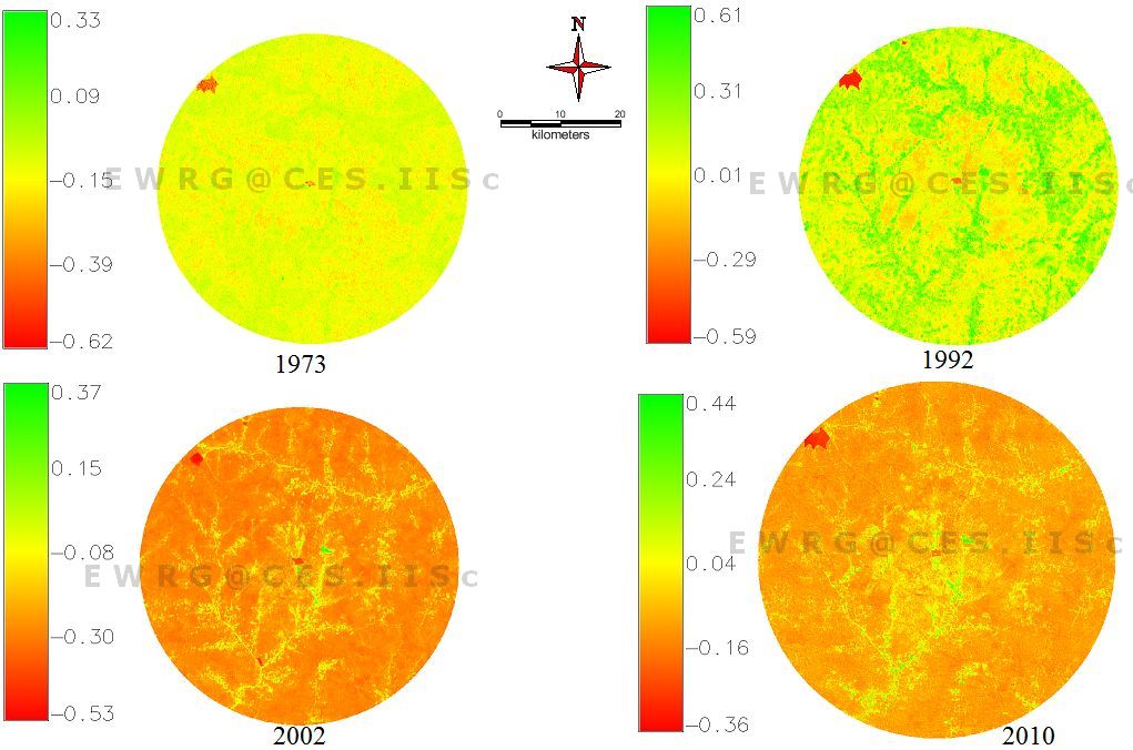
Vegetation cover of the study area assessed through NDVI (Figure 4) shows that area under vegetation has declined by about 19%. Temporal NDVI values are listed in Table 4, which shows that there has been a substantial increase in the area other than the vegetation.
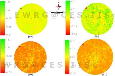
Figure 4: Temporal Land cover changes during 1973 – 2009
Table 4: Temporal Land cover
| Year |
Vegetation |
Non vegetation |
| % |
% |
| 1973 |
98.01 |
1.99 |
| 1992 |
94.72 |
5.28 |
| 2002 |
91.33 |
8.67 |
| 2010 |
79.41 |
20.57 |
1.2 Land use analysis
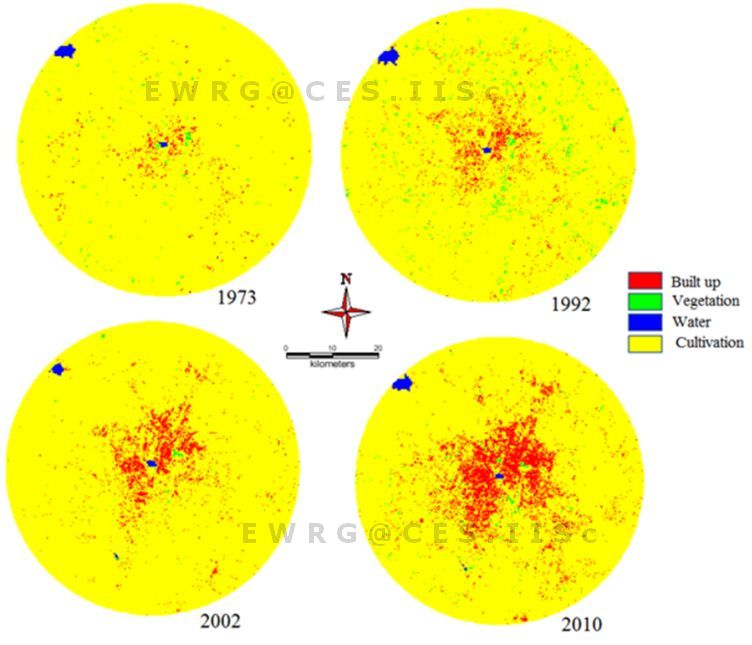
Land use assessed for the period 1973 to 2010 using Gaussian maximum likelihood classifier is listed table 5 and the same is depicted in figure 5. The overall accuracy of the classification Ranges from 73.23% (1973) to 94.32% (2010). Kappa statistics and overall accuracy was calculated and is as listed in Table 6. There has been a significant increase in built-up area during the last decade evident from 21% increase in urban area. Other category also had an enormous decrease in the land use. Consequent to these, vegetation cover has declined during the past four decades.
Table 5: Temporal land use details for Gulbarga
| Land use |
Urban |
Vegetation |
Water |
Cultivation and others |
| Year |
| 1973 |
1.08 |
1.01 |
0.34 |
97.17 |
| 1992 |
2.62 |
1.54 |
0.40 |
95.44 |
| 2002 |
7.22 |
0.55 |
0.23 |
92.01 |
| 2010 |
22.52 |
0.49 |
0.39 |
76.60 |
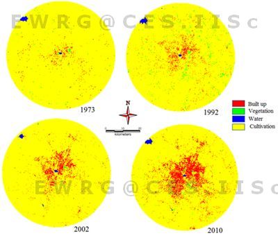
Figure 5: Classification output of Gulbarga
Table 6: Kappa statistics and overall accuracy
| Year |
Kappa coefficient |
Overall accuracy (%) |
| 1973 |
0.72 |
73.23 |
| 1989 |
0.86 |
89.69 |
| 1999 |
0.82 |
81.47 |
| 2009 |
0.93 |
94.32 |
1.3 Urban sprawl analysis
Shannon entropy computed using temporal data are listed in table 7. Gulbarga is experiencing the sprawl in all directions as entropy values are closer to the threshold value (log (10) = 1). Lower entropy values of 0.018 (SW), 0.023 (SE) during 70’s shows an aggregated growth. However, the region show a tendency of dispersed growth during post 2000 with higher entropy values 0.268 (NE), 0.212 (NW) in 2010. Shannon's entropy values of recent time indicate of minimal but fragmented/dispersed urban growth in the region.
Table 7: Shannon Entropy Index
|
NE |
NW |
SE |
SW |
| 2010 |
0.268 |
0.212 |
0.193 |
0.141 |
| 2002 |
0.139 |
0.112 |
0.091 |
0.098 |
| 1992 |
0.086 |
0.065 |
0.046 |
0.055 |
| 1973 |
0.067 |
0.034 |
0.023 |
0.018 |
1.4 Spatial patterns of urbanisation
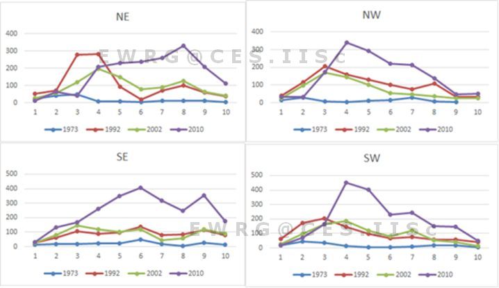
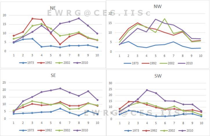
Further to understand the spatial pattern of urbanization and the dynamical growth, eight landscape level metrics were computed zonewise for each circle. These metrics are discussed below: Number of Urban Patch (Np) is a landscape metric indicates the level of fragmentation and ranges from 0 (fragment) to 100 (clumpiness). Figure 6a illustrates of the urban growth evident from the increase in number of patches in 1992 and 2002 whereas in 2010 the patches have decreased indicating aggregation or clumped growth, while outskirts and boundary area (5th circle onwards) is showing a fragmented growth. Clumped patches at center are more prominent in NE and SE directions. Outskirts are fragmented more in NE and SE directions indicative of higher sprawl in the region.
NOTE: X-axis represents gradients and Y-axis value of the metrics
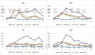
Figure 6a: Number of urban patches (zone, circlewise)
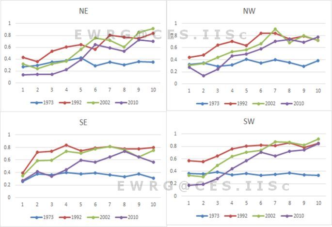
The patch density (Figure 6b) is calculated on a raster data, using a 4 neighbor algorithm. Patch density increases with a greater number of patches within a reference area. Patch density was higher in 1992 in all directions and gradients due to small urban patches. This remarkably increased in 2002 in the outskirts which are an indication of sprawl in 2002, subsequently increasing in 2010. PD is low at centre indicating the clumped growth, which was in accordance with number of patches.
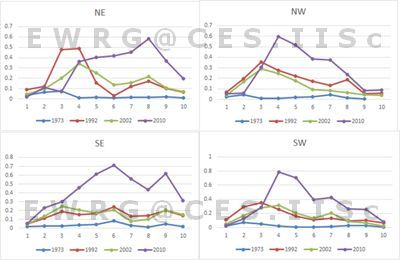
Figure 6b: Patch density – zone, circle wise
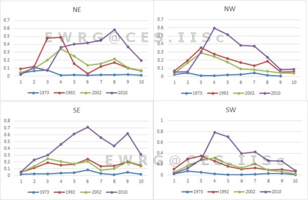
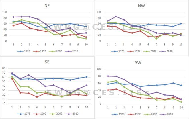
Landscape Shape Index (LSI): LSI equals to 1 when the landscape consists of a single square or maximally compact (i.e., almost square) patch of the corresponding type and LSI increases without limit as the patch type becomes more disaggregated. Figure 6c indicates of lower LSI values in 1973 due to minimal concentrated urban areas at the center. The city has been experiencing dispersed growth in all direction and circles since 1990’s. In 2010 it shows a aggregating trend at the centre as the value is close to 1, whereas it is very high in the outskirts indicating the peri urban development.
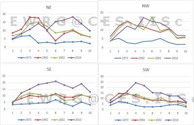
Figure 6c: Landscape Shape index – zone andcirclewise
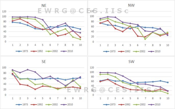
Normalized Landscape Shape Index (NLSI): NLSI is 0 when the landscape consists of Single Square or maximally compact almost square, it increases as patch types becomes increasingly disaggregated and is 1 when the patch type is maximally disaggregated. Results (Figure 6d) indicates that the landscape in 2010 had a highly fragmented urban class in the buffer region and is aggregated class in the center, conforming to the other landscape metrics. Clumpiness index equals zero when the patches are distributed randomly, and approaches 1 when the patch type is maximally aggregated. Aggregation index equals 0 when the patches are maximally disaggregated and equals 100 when the patches are maximally aggregated into a single compact patch.
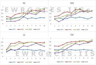
Figure 6d: Normalised Landscape Shape index – zone and circlewise
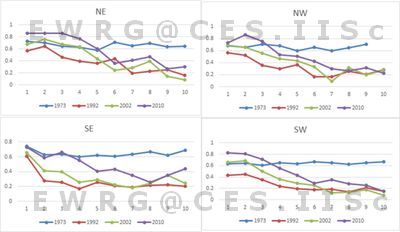
Figure 6e: Clumpiness – zonewise, circle wise
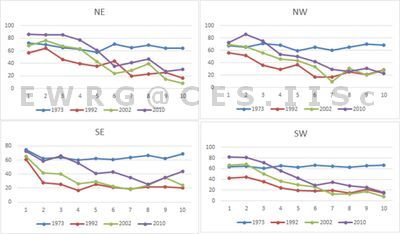
Figure 6f: Aggregation-zone and circle wise
Percentage of Like Adjacencies (Pladj) is the percentage of cell adjacencies involving the corresponding patch type those are like adjacent. Cell adjacencies are tallied using the double-count method in which pixel order is preserved, at least for all internal adjacencies. This metrics also indicates (Figure 6g) the city center is getting more and more clumped and the adjacent patches of urban are much closer and are forming a single patch in 2010 and outskirts are relatively sharing different internal adjacencies are the patches are not immediately adjacent which is also indicative of sprawl. Patch cohesion index measures the physical connectedness of the corresponding patch type. This is sensitive to the aggregation of the focal class below the percolation threshold. Patch cohesion increases as the patch type becomes more clumped or aggregated in its distribution; hence, more physically connected. Above the percolation threshold, patch cohesion is not sensitive to patch configuration. Figure 6h indicate of physical connectedness of the urban patch with the higher cohesion value (in 2010). Lower values in 1973 illustrate that the patches were rare in the landscape.
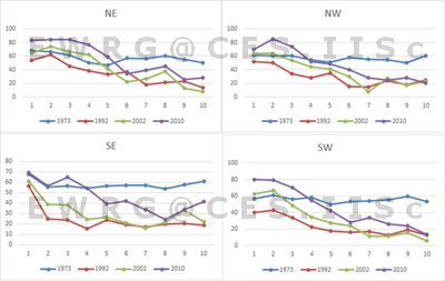
Figure 6g: Zone and circle wise – Pladj
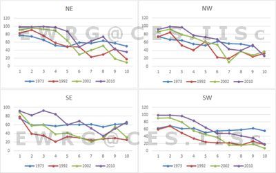
Figure 6h: Cohesion Index
|