Materials and Methods

Study area

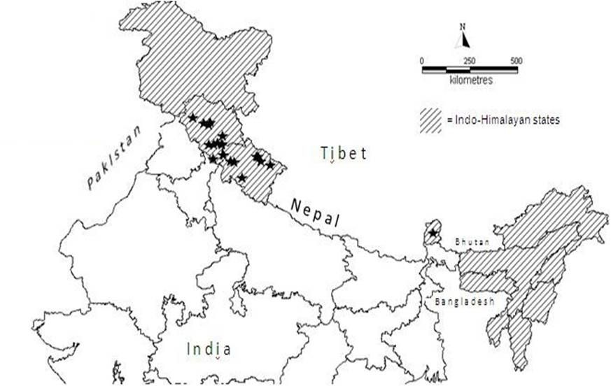
Indian Himalayan Region (IHR) ranges from Jammu & Kashmir to Arunachal Pradesh including Himachal Pradesh, Uttarakhand, Sikkim, Darjeeling district of West Bengal. North East states (i.e. Assam, Meghalaya, Manipur, Nagaland, Mizoram and Tripura) are also included as part of eastern Himalaya as per available literature (Samant et al., 1998; WWF-US, 2005) (Fig 1.).

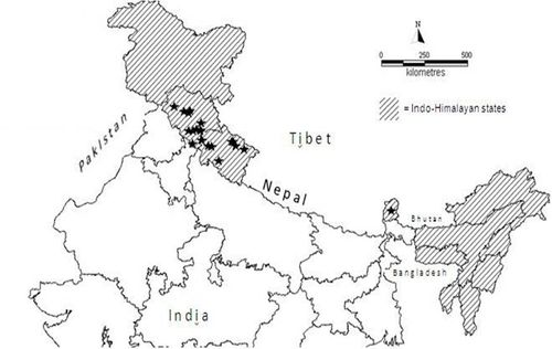
Fig. 1. Study area : Indo – Himalayan Region  (     = occurrence points for B.aristata)

Species occurrence data

Twenty one occurrence points of Berberis aristata were shortlisted from a collection of field survey done at Moolbari watershed area of Himachal Pradesh, India  and secondary data available from published literatures (Uniyal, 2002; Chhetri et al., 2005 and Anonymous, 2007-2008) (Fig 1.). Moolbari watershed is situated in Shimla district, Himachal Pradesh, India and encompasses an area of 13.41 sq. km from 31.07-31.17 ^oN and 77.05-77.15 ^oE. Field study was conducted by following standard ecological methods and the species was identified with the help of keys (published flora) in addition to the consultation of herbarium samples and discussion with the Himalayan flora experts.

Environmental data

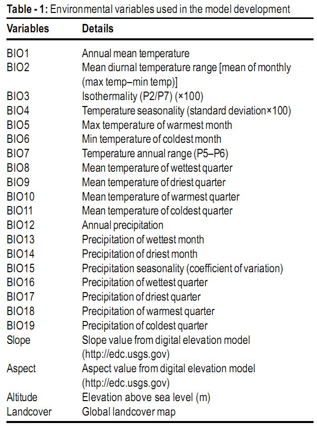
For environmental information, 19 bioclimatic variables derived from globally interpolated datasets (source: http://www.worldclim.org) representing annual trends, seasonality and extreme or limiting environmental factors, were used for the modelling study which are presumed to be maximum relevant to plant existence (Pearson and Dawson, 2003; Irfan Ullah et al., 2007). The WorldClim climate layers were created by interpolating observed climate from climate stations around the world, using a thin-plate smoothing spline set to a resolution of approximately 1 km, over the 50-year period from 1950 to 2000 (Hijmans et al., 2005). Additioinally, we used aspect, slope, altitude (http://edc.usgs.gov/products/elevation/gtopo30/hydro/asia.html and  http://www.worldclim.org) and landcover (GLC 2000), in the model development (Table 1).  All analyses were conducted at the 1 x 1 km pixels spatial resolution of the environmental data sets since, bioclimatic variables with finer than 1 km resolution is not available at this moment. All environmental data layers were finally cropped for the study area (Indian Himalayan Region) to perform the modeling experiment.

Table 1. Environmental Variables used in the model development

Model development-

We followed three different modeling techniques for our study. The open Modeller desktop version 1.0.9 was used for GARP (GARP with best subsets – Desktop GARP implementation) and Bioclim techniques. Maxent 3.3.1 used for performing Maxent algorithm (downloaded from http://www.cs.princeton.edu/~schapire/maxent/). A brief description of the techniques is mentioned below.

GARP is a genetic algorithm that creates ecological niche models for species. The models describe environmental conditions under which the species should be able to maintain populations. For input, GARP uses a set of point localities where the species is known to occur and a set of geographic layers representing the environmental parameters that might limit the species' capabilities to survive. Details of the modeling algorithm can be found in Stockwell and Peters, 1999. In our study, we assigned 50% of the occurrence points as training data for developing the model while rest of the data has been used as intrinsic test data.  For other parameters, we used default values available in open Modeler i.e. commission threshold = 50% of distribution models, omission threshold = 20% of the models with least omission error and resample value = 2,500.

Bioclim is one of the earlier modeling techniques, tallying species occurrence points for each environmental variable including 95% of the distribution (i.e. excluding extreme 5% of the distribution) along each ecological dimension. Details of the algorithm can be obtained from Busby (1991).

The maximum entropy (MaxEnt) approach estimates a species' environmental niche by finding a probability distribution that is based on a distribution of maximum entropy (with reference to a set of environmental variables) (Phillips et al., 2006). Default values of different parameters, maximum iterations = 500, convergence threshold = 0.00001 and 50% of data points were used as random test percentage in our study.

Model validation -

Prediction accuracy of all three model outputs was measured through receiver operating characteristics (ROC) analysis because of its wider application in the modeling studies despite some recent arguments (Lobo et al., 2008; Boubli and Lima, 2009; VanDerWal et al., 2009; Yates et al., 2010). ROC plot can be generated by putting the sensitivity values, the true positive fraction against the false positive fraction for all available probability thresholds. A curve which maximizes sensitivity against low false positive fraction values is considered as good model and is quantified by calculating the area under the curve (AUC). An AUC statistic closer to1.0 indicates total agreement between the model and test data and considered as good model. An AUC with value closer to 0.5 considered to be no better than random.