 |
Modelling landscape dynamics with LST in protected areas of Western Ghats, Karnataka |
 |
bCentre for Sustainable Technologies (astra), Indian Institute of Science, Bangalore, Karnataka, India
cCentre for infrastructure, Sustainable Transportation and Urban Planning (CiSTUP), Indian Institute of Science, Bangalore, Karnataka, India
1Web URL: http://ces.iisc.ac.in/energy; http://ces.iisc.ac.in/foss.
*Corresponding author: emram.ces@courses.iisc.ac.in (T.V. Ramachandra).
|
Materials and method 2.1. Study area The Western Ghats is one among the 35 global hotspots of biodiversity and it lies in the western part of peninsular India in a series of hills stretching over a distance of 1600 km from north to south and covering an area of about 1,60,000 sq.km. It harbors very rich flora and fauna and there are records of over 4600 species of flowering plants with 38% endemics, 330 butterflies with 11% endemics, 197 reptiles with 52% endemics, 529 birds with 5% endemics, 161 mammals with 12% endemics, 343 fishes with 39% endemics and 248 amphibians with 62% endemics (http://wgbis.ces.iisc.ac.in/biodiversity/). Unplanned developmental activities during the post-industrialization period have threatened biodiversity, ecology and water availability. In this context, the government of India has created PAs network across wild habitats in order to conserve and reduce impacts. Fig. 2 depicts the locations of Kudremukh National Park (KNP), Rajiv Gandhi Tiger Reserve (RTR), Bandipur Tiger Reserve (BTR), which were chosen to understand the status of forests and LU dynamics. KNP comes under the Global Tiger Conservation Priority-I (as per Wildlife Conservation Society (WCS) and World Wide Fund-USA) and is a habitat to diverse endemic tax. RTR is also known as Nagarahole National Park, sensitive habitat to elephants (connects to Nilgiri Biosphere Reserve), and has been experiencing anthropogenic pressure, evident from degradation of forests, intensified agricultural activities. BTR is the first NP to get status as tiger reserve (TR) in 1973, which is also a habitat for numerous bird species (~250 species) and mammals endemic to Western Ghats. Rampant habitat degradations are common phenomenon across PAs due to unplanned developmental projects such as dams and interstate highways in the ecologically sensitive habitats apart from other pressures such as grazing, firewood collection and weed infestation (Eupatorium, Parthenium, Chromolaena odorata), illegal hunting, poaching (elephant poaching for ivory), etc. due to lack of effective ecomanagement leading to a very frequent instances of humananimal conflicts. Unauthorized occupation of forest lands for cultivation in the buffer region has aggravated human-animal conflicts leading to the frequent animal mortalities.
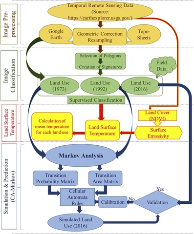
Fig. 2. Study area - select protected areas of Western Ghats, Karnataka. 2.2. Method Mapping, monitoring, modelling and visualization of LULC dynamics in the select protected areas with 10 km buffer in the central Western Ghats has been carried out as discussed in Fig. 3. Remote sensing (RS) data used in the study are Landsat MSS (1973), TM (1992), OLI8 (2016), IRS p6L4X (2016), and online Google Earth data (http://earth.google.com). Topographic maps have provided ground control points to rectify RS data and scanned paper maps. Survey of India (SOI) toposheets (1:50000 and 1:250000 scales) and vegetation map of South India developed by French Institute (1986) of scale 1:250000 was digitized to identify various forest cover types and temporal analyses to find out the changes in vegetation. Pre-calibrated GPS (Global Positioning System - Garmin GPS unit) used for field measurements. Land use analyses involved
Fig. 3. Protocol for mapping, monitoring, modelling and visualization of LULC dynamics. LST is estimated pixel-wise across varied land use categories as per the standard protocol (Bharath et al., 2013) based on each land use class emissivity that considers the amount of thermal infrared energy radiated from the Earth's surface of many different types of Earth surface processes, surface-atmosphere interactions. Estimation of LST using emissivity will provide more accurate estimation with appropriate calibration of atmospheric contamination by a separation of surface emissivity and temperature from radiance at ground level and atmospheric corrections (Li et al., 2013; Zak and O stir, 2012; Mohamed et al., 2017 Inamdar et al., 2008; Merlin et al., 2010). Emissivity is an intrinsic property of the surface, potential for enhancing ability to monitor landscape changes in environmentally sensitive zones as compared to other congruent practices (Hulley et al., 2014). The surface temperature of the area is calculated as per equation (3), through equations (1) and (2).
Lλ represents the top of atmosphere spectral radiance (Watts/ (m2 srad μm)). λ represents the wavelength of the thermal band. Qcal is the DN value of the pixel under consideration. AL and MLare offset and gain factor respectively whose value for TM is AL = 1.238, ML = 0.055 and OLI is AL= 0.1, ML = 3.3420 * 10-4. K1 (Watts/(m2 srad mm)) and K2 (kelvin) represents the pre-launch calibration coefficients. Value of K1 is 607.76 and K2 is 1260.56 (for TM), while K1 for OLI (Band 11) is 480.8883 and K2 for is 1201.1442. TB represents the At-satellite brightness temperature. Emissivity correction is carried out using surface emissivity for the specified LC derived from the methodology described in (Stathopoulou et al., 2007. The emissivity corrected land surface temperature (Ts) is computed from equation (3).
where, λ is the wavelength of emitted radiance for which the peak response and the average of the limiting wavelengths (l = 11. 5 mm) were used, ρ = h * c/σ (1.438 *10-2 mK), σ = Stefan Boltzmann's constant (5.67 *10-8 Wm- 2 K-4 =1.38 * 10-23J/K), h = Planck's constant (6.626 * 10-34Jsec), c = velocity of light (2.998 * 108m/sec), and ε is spectral emissivity.
where, P(N) is state probability of any times, and P (N-1) is preliminary state probability. Transition area matrix can be obtained by,
ij is the sum of areas from the ith land use category to the jth category during the years from start point to target simulation periods, and n is the number of land use types. The transition are a matrix must meet the following conditions
Citation : Ramachandra T V, Bharath Settur, Nimish Gupta, 2017. Modelling landscape dynamics with LST in protected areas of Western Ghats, Journal of Environment Management (In PRESS)
|
||||||


 .............................(1)
 .............................(2)
 .............................(3)
 .............................(4)
 .............................(5)
 .............................(6)