Study area

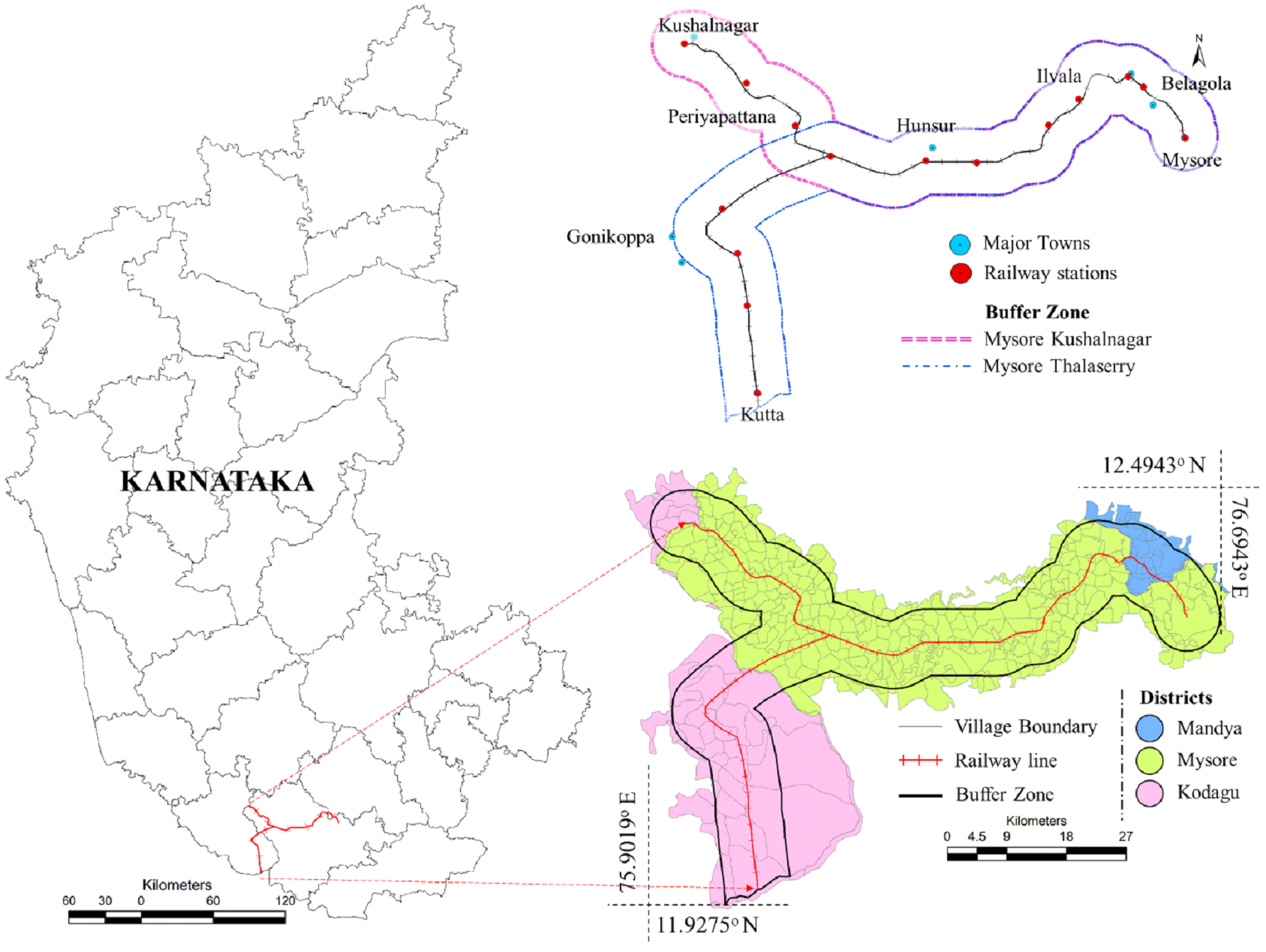
The study region is located in the Western Ghats (one among 36 global biodiversity hotspots), which extend along the west coast of India with pristine and fragile ecosystems (Subash Chandran 1997; Gunnel and Radhakrishna 2001; Daniels and Venkatesan 2008). The study region supports exceptional endemic biodiversity, benefiting both society and the environment due to various goods and services. The hydrological and watershed services are evident from the water provision sustaining dometic and irrigation requirements in peninsular India. The soil and water of this region sustain the livelihoods of millions of people. These fragile ecosystems are under threat due to the implementation of unplanned short-sighted developmental projects, which are escalating anthropogenic activities (Ramachandra et al. 2020). Globalization and consequent relaxation in Indian markets have given impetus to the implementation of numerous industries and linear infrastructure projects. Implementation of these projects would alter the hydrologic regime (floods and droughts), induces instability in the landscape (leading to frequent landslides and mud slides), impacts wild life habitats, hinders movement paths, foraging areas, increases mortality of wild animals (Borda-de-Água et al. 2017; Gilhooly et al. 2019) and enhance the episodes of human-animal conflicts. Infrastructure projects proposed in this region are railway connectivity between i) Mysore Kushalnagar and ii) Mysore Thalassery, which originates from Mysore district and passes through Western Ghats (Fig. 1 and Table 2). A buffer zone of 5 km on either side of the proposed railway lines was considered to understand the projects' influence on landscape and wildlife habitat/presence zones within Karnataka state. The buffer zone covers about 452 villages in the districts of Mysore (347), Kodagu (62) and Mandya (43).

Table 2. Details of the proposed railway projects

Fig. 1. Study Area

3. Data and Method

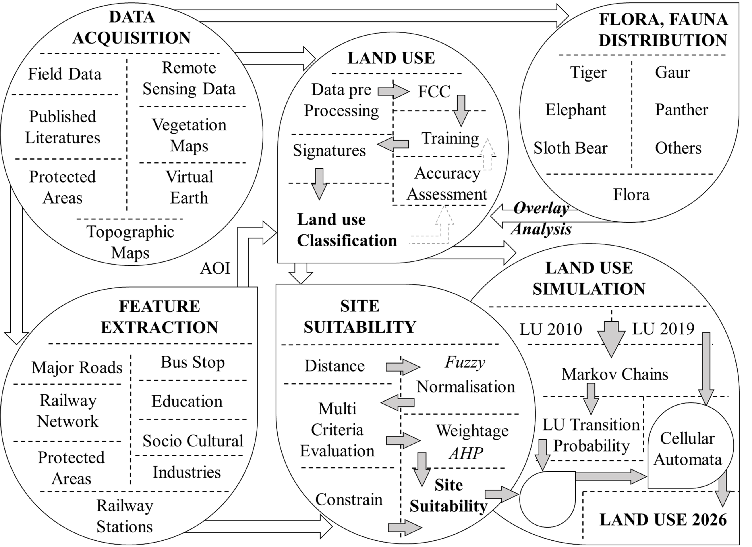
The process toward understanding land use dynamics and impact on ecology in the study region (of linear railway projects) involved i) data collection and analyses, ii) land use analysis, iii) visualization of likely land-use changes, and iv) spatial patterns of biodiversity (Fig. 2).

3.1. Data Collation

This involved collecting (i) primary data from the field and (ii) secondary data from the government agencies and virtual data portals. Table 3 describes the various data used in the analysis. The cloud-free temporal remote sensing data IRS LISS 3 sensor for the years 2010 and 2019 was obtained from NRSC (National Remote Sensing Centre). Field data was collected using a pre-calibrated handheld Global Positioning System (GPS) at various locations along (and beyond) the study area aided as ground truth data (training data) that has helped in geo-rectification and classification of remote sensing data. This data is supplemented with the information from vegetation map (Pascal 1986), topographic maps (Survey of India 2018a) and virtual earth portals such as Bhuvan (National Remote Sensing Centre 2016) and Google Earth (Pascal 1986; National Remote Sensing Centre 2016; Survey of India 2018a; Google 2020)

Table 3. Data and source

3.2 Land use analysis

Remote sensing data was preprocessed to rectify geometric error using ground control points obtained from field and virtual earth databases portal. Radiometric correction is done to enhance the scene radiometric properties (contrast enhancement) for better visual interpretation of the data (Jensen 1996; Lillesand et al. 2004; Gonzalez and Woods 2007). Training data (ground truth data) was collected from the field and supplemented with the secondary data covering over 15% of the study area. Gaussian Maximum likelihood classifier was used to classify the remote sensing data into six land use classes (Table 4) using 60% of the training data (Bharath et al. 2018c). Accuracy of the land use classification was assessed through kappa statistics and computation of overall accuracy (Congalton and Green 2009), considering 40% of the training data. Figure 2 outlines the protocol adopted to assess and visualise landscape dynamics.

Fig. 2. Method for assessing the landscape dynamics

Table 4. Land use classes and associated features

3.3 Visualisation of land use dynamics through simulation and modeling

Agent-based modeling technique by combining various spatial and mathematical aspects of Fuzzy logic, Boolean algebra, analytical hierarchical process (AHP), multi-criteria evaluation (MCE), cellular automata (CA), and Markov chains have been used to predict the likely land uses. ABM has proved to be a reliable, individual decision-making tool to capture spatial dynamics by incorporating socio-economic and environmental factors (Matthews et al. 1999; Hosseinali et al. 2013; Bharath et al. 2016a, 2018b).

Factors contributing to land-use changes along the proposed railway network are city centers, major roads, educational institutions, bus stops, industries and railway stations. Similarly, factors inhibiting land-use change considered are protected areas (forest department), lakes, and river course was derived from the secondary databases (government agencies of the spatial extent, etc.). Distance maps were prepared for each of the contributing factors and Boolean maps for each of the constrain (0 represented no change, 1 represents space that can change). Distance from each of the factors were overlaid on individual land use to determine the effective distance of influence. Fuzzy Logic (Zadeh 1965) was used to understand the behavior of agents of growth across various land use classes and normalize the influences (Eastman 2012) between 0 and 1.

The distance of influence of each agent with a different degree of membership and representation function are measured and provide input to AHP weighing process, aided in multi-criteria decision making. Multi-criteria evaluation was used to compare the influence of each of the factors on land-use change, based on expert opinion using analytical hierarchical process (AHP) (Kardi 2005; Gorsevski et al. 2012). Weights for different factors obtained from AHP and constrain maps as Boolean are used to derive site suitability maps using MCE (Li et al. 2013; Dapueto et al. 2015).

A response matrix is generated to measure the relative dominance of item i over item j with the decision maker’s assessments a_ij, that follow a uniform probability distribution.

…… Eq. 2

where W_i and W_j are the priority weights and = 1, is inconsistency observed in the analysis. The comparison matrix elements were compared pairwise to relate a single element at the level directly and ranked by eigenvector of the matrix (Zhang et al., 2015) and eigenvalue of is computed (Ying et al., 2007). A new vector is obtained by multiplying pairwise comparison matrix and eigenvectors (Eq 3, 4). The consistency of weightages is evaluated through Consistency Index (CI) (Eq. 5).

………..Eq. 3

….. Eq.4

……… Eq. 5

where CI is the consistency index, 𝜆_𝑚𝑎𝑥 is the largest or principal eigenvalue; n is the order of the matrix. If CI = 0, the matrix had a complete consistency. The worse consistency will represent greater value of CI.

…….Eq. 6

where RI is the average of the resulting consistency index (Random Index) depending on the order of the matrix. If CR value is less than 0.10, the matrix had a reasonable consistency, otherwise, the matrix should be altered for better CR. Markov chains are statistical models used to predict the likely changes in the landscape from current state (S(t)) to future state (S(t,t+1)) based on transition probability () of land use from one class to another (earlier to current) (Hamad et al. 2018). Mathematically Markov chain is given as Eq.7

………..Eq. 7

Cellular automata determines the state of each cell in the data, based on the cell state, neighborhood, rule dependencies (Bharath et al. 2016b; Gidey et al. 2017). These rule dependencies are derived based on the Markov chains and the site suitability maps obtained from AHP (Gidey et al. 2017; Bharath et al. 2018a; Ramachandra et al. 2019b). Site suitability maps, Markov chains and Cellular Automata (CA) were integrated to visualize the landscape change patterns for the year 2026.

3.4 Distribution of Flora and Fauna.

Distribution of flora (Ramachandra et al. 2016; Shankar 2016) and fauna such as tiger (Panthera tigris), panther (Panthera pardus), sloth bear (Melursus ursinus), gaur (Bos gaurus), Asian elephant (Elephas maximus) were collated from publications of the Karnataka Forest Department (KFD 2018), National Tiger Conservation Authority (Jhala et al. 2011, 2019), Wildlife Institute of India, other published literatures (Madhusudan et al. 2015) and through field investigations. Spatial patterns of land-use and distribution of flora and fauna were compared to understand the possible regions of anthropogenic influence on biodiversity.