Materials and methods
Study area: Indian city Kolkata, the capital West Bengal has been considered for the analysis. Kolkata is located in the eastern part of India and is situated on the eastern bank of Hooghly River, adjacent to Assam, Sikkim and borders of Bangladesh (Bunting et al., 2002). Kolkata is the third most populous city in India, 13th most populous and eighth largest urban agglomeration city in the world, having a population of approximately 14.11 million (Census, 2011). Its population density has increased from 2039 persons per sq. km (in 1971) to 3879 persons per sq. km (in 2011) (Table 1). Kolkata lies at 22°34’N and 88°24’E. It is at an altitude of 6 m above mean sea level and a distance of 96 km from the Bay of Bengal. Its temperature ranges from 12OC to 27OC in winters and 24OC to 38OC in summers. The average rainfall is about 160cm which keeps the city cool after a hot summer (Bunting, et al., 2002). Kolkata has mainly alluvial soil and the main crops/plantations cultivated are rice, jute, mango, coconut, jackfruit, guava, and black berries. Kolkata is an important centre for art, literature, architecture and cultural heritage. Thriving since the pre-colonial age, Kolkata has preserved many of its beautiful monuments, sculptures, and historical buildings, a prominent one of which is the renowned Indian Museum that was established in 1814, which today, is considered as the oldest museum in Asia. Kolkata is considered a historical landmark that had laid the foundations for quite a few British monuments such as the Marble palace and the Victoria Memorial. Kolkata was once the capital of India during the British rule, but in 1911, it lost that status to Delhi due to its improper geographic location in India. Due to rapid urbanization in the current years, Kolkata is now facing problems such as traffic congestion and pollution. Kolkata is one of the major commercial and financial hubs of northeastern India. In 2009, Kolkata’s GDP was about 162 billion which made it the third highest among all Indian cities. Its industries largely produce engineering products, electronic components, electrical equipment, textiles, jewelry, chemicals, tobacco, food products, and jute products, all of which add significantly to the economic development of the city. Information Technology industries also play a prominent role in adding to its economic growth by attracting many software and telecoms firms from across the country as well as from the rest of the world. The GDP of Kolkata is about $150 Billion which make the economically strong than compared to others cities except Mumbai and Delhi.
Urban Development planning and infrastructure: The Kolkata Metropolitan District is a planning unit of Kolkata that covers three municipal corporation units, 34 municipalities and the Greater Kolkata on the whole (Bonnerjee S, 2012). The urban planning development of Kolkata is undertaken by the Kolkata Municipal Corporation (KMC) which constitutes the administrative core of the city while the planning for the wider agglomeration surrounding Kolkata Municipal Corporation is undertaken by Kolkata Metropolitan Authority (Gregory, 2005). KMC is responsible for the infrastructural development and the administration of the city. Kolkata Metropolitan Development Authority (KMDA) is the development authority for the Kolkata Metropolitan Area (KMA). The KMDA also undertakes city planning, creates townships, and develops infrastructure in the city. The planning begins with the gathering of information about a particular location in a systematic manner. Due to rapid urbanization in the city, planning becomes a challenging task with constraints such as high rates of pollution, dispersed growth at outskirts (per-urban regions), traffic congestion, and reduced green spaces, open spaces and small lakes. In order to understand the urban dynamics, Kolkata city has been analysed by considering administrative boundaries with 10 km buffer (Figure 1).
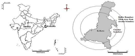
Figure 1: Study area - Kolkata administrative boundary with 10 km buffer.
Kolkata is a highly populated city in India that has a population of 14.11 million as per provisional census of 2011. Figure 2 describes the temporal increase in population during the last 100 years.
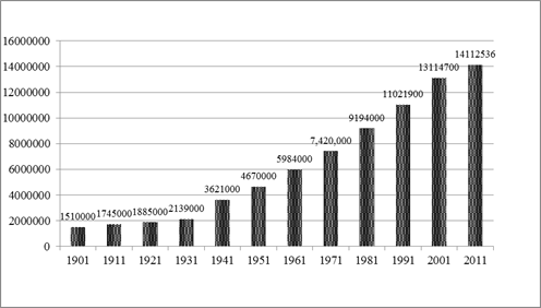
Figure 2: Population growth since 1901 (Source: Census of India).
City |
Area
(sq. km.) |
Year |
Population |
Population Density
(Persons per sq.km.) |
Kolkata |
3638.49 |
1971 |
7420000 |
2039 |
1981 |
9,030,000 |
2482 |
1991 |
10,890,000 |
2993 |
2001 |
13,217,000 |
3632 |
2011 |
14,112,536 |
3879 |
Table 1: Population growth in Kolkata during 1971- 2011
Data: Urban dynamics was analysed using temporal remote sensing data for the period between 1973 and 2010. The time series spatial data acquired from Landsat Series Multispectral sensor (57.5m) and thematic mapper (28.5m) sensors for the period between 1979 and 2010 were downloaded from a public domain (http://glcf.umiacs.umd.edu/data) as indicated in Table 2. Base layers and training data (for classifying remote sensing data) were derived from the Survey of India (SOI) topographic maps of scales 1:250000 and 1:50000. Features such as extent of water bodies, certain roads etc., were derived from 1:50000 map, while 1:250000 was used mainly for training data. Further, these layers were resampled to 30 m.
DATA |
Year |
Purpose |
Landsat Series Multispectral sensor(57.5m) |
1979 |
For Land cover and Land use analysis |
Landsat Series Thematic mapper (28.5m) and Enhanced Thematic Mapper sensors |
1990,1999, 2010 |
For Land cover and Land use analysis |
Survey of India (SOI) toposheets of 1:50000 and 1:250000 scales |
|
To generate boundary and base layer maps. |
Field visit data –captured using GPS |
|
For geo-correcting and generating validation dataset |
Table 2: Data used in the Analysis
Data Analyses: Figure 3 outlines the process of data analyses, which includes preprocessing, analysis of vegetation cover and land use, and lastly, the gradient wise zonal analysis of Kolkata using landscape metrics.
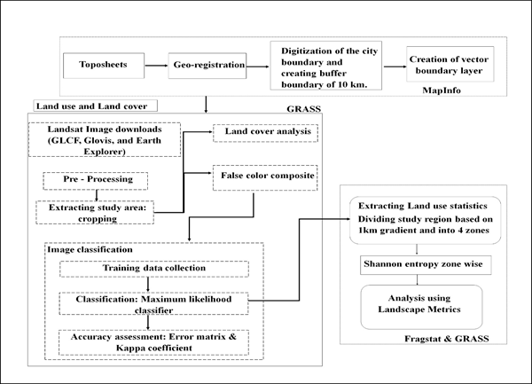
Figure 3: Procedure adopted for classifying landscape and computation of metrics.
-
Preprocessing: Remote sensing data (Landsat series) for Kolkata of different time periods were downloaded from Global Land Cover Facility (http://www.glcf.umd.edu/index.shtml and http://www.landcover.org/), United States Geological Survey (USGS) Earth Explorer (http://edcsns17.cr.usgs.gov/NewEarthExplorer/) and Glovis (http://www.glovis.usgs.gov). The remote sensing data obtained were geo-referenced, geo-corrected, rectified and cropped with respect to the study area. Geo-registration of remote sensing data (Landsat data) was done using ground control points collected from the field using pre-calibrated GPS receiver (Global Positioning System) and also from known points (such as road intersections, etc.) collected from geo-referenced topographic maps published by the Survey of India. The Landsat satellite data of 1979 (with spatial resolution of 57.5 m x 57.5 m (nominal resolution)) and that of 1989 - 2010 (with spatial resolution of 28.5 m x 28.5 m (nominal resolution)) were resampled to 30m each in order to maintain uniformity in spatial resolution across different time periods. The study area included the Kolkata administrative area with 10 km buffer.
- Vegetation cover analysis: Vegetation cover analysis was performed to understand the changes in the land cover (area under vegetation and non-vegetation) during 1979-2010. Normalised difference vegetation index (NDVI) was found suitable and was used for measuring vegetation cover (Ramachandra et al., 2012; http://wgbis.ces.iisc.ac.in/energy/paper/comparitive/methodlogy.htm). NDVI values ranges between -1 to +1. Very low values of NDVI (-0.1 and below) correspond to non-vegetation (soil, sand, urban built up, etc.), whereas 0 indicates water cover. Moderate values represent low density vegetation (0.1 to 0.3), whereas high values indicate thick canopied vegetation (0.6 to 0.8).
- Land use analysis: The method involves i) generation of False Colour Composite (FCC) of remote sensing data (bands – green, red and NIR). This helped in locating heterogeneous patches in the landscape, ii) selection of training polygons (corresponding to heterogeneous patches in FCC) covering 15% of the study area that were uniformly distributed over the entire study area, iii) loading these training polygons co-ordinates into pre-calibrated GPS receiver. Pre – calibration involved range corrections by finding the shift (if any) of locations (with GPS receiver) and known ground control points (derived from survey benchmarks, topographic maps). Range correction constitute an important component as most of the GPS receivers have an error of 2-10 m, iv) collection of the corresponding attribute data (land use types) for these polygons from the field. GPS receiver helped in locating respective training polygons on the field, v) supplementing this information with Google Earth, and vi) using 60% of the training data for classification, while using the rest for validation or accuracy assessment.
Land use analysis was carried out using supervised pattern classifier - Gaussian maximum likelihood algorithm. Remote sensing data was classified using signatures from training sites that include all the land use types detailed in table 3. Mean and covariance matrix were computed using estimates of maximum likelihood estimator. Maximum Likelihood classifier is used to classify the data using these signatures generated. This technique is proven to be a superior classifier as it uses various classification decisions using probability and cost functions (Duda et al., 2000, Ramachandra et al., 2012). Mean and covariance matrix are computed using estimates of maximum likelihood estimator. Land uses during different time periods were estimated using the temporal data through open source program GRASS - Geographic Resource Analysis Support System (http://ces.iisc.ac.in/grass). Signatures were collected from field visits and with the help of Google Earth. 60% of the total generated signatures were used in classification, and 40% signatures were used in validation and accuracy assessment. Classes of the resulting image were reclassified and recoded to form four land-use classes. The noise in the classified image of 1973 was removed by smoothing filter (3 X 3 median filters).
Land use Class |
Land uses included in the class |
Urban |
Residential areas, industrial areas, and all paved surfaces and mixed pixels having built up area. |
Water bodies |
Tanks, Lakes, Reservoirs. |
Vegetation |
Forest, Cropland, nurseries. |
Others |
Rocks, quarry pits, open ground at building sites, unmetalled roads. |
Table 3: Land use classes
-
Accuracy assessment: These methods evaluate the performance of classifiers (Mitrakis et al., 2008). This is done through comparison of kappa coefficients (Congalton et al., 1983), which are common measurements used to demonstrate the effectiveness of the classifications (Congalton, 1991; Lillesand & Kiefer, 2002). Recent remote sensing data (2010) were classified using the collected training samples. Statistical assessment of classifier performance, based on the performance of spectral classification considering reference pixels, was done which included computation of kappa (κ) statistics and overall (producer's and user's) accuracies. For earlier time data, training polygon along with attribute details were compiled from earlier published topographic maps, vegetation maps, and revenue maps.
- Zonal Analysis: City boundary along with the buffer region was divided into 4 zones: North east (NE), Southwest (SW), Northwest (NW), and Southeast (SE) for further analysis as urbanization is not uniform in all directions. As most of the definitions of a city or its growth is defined in terms of directions, it was considered more appropriate to divide the regions into 4 zones based on directions. Zones were divided considering the Central pixel (Central Business district). The growth of the urban areas along with the agents of changes is understood in each zone separately through the computation of urban density for different periods.
Division of zones into concentric circles (Gradient Analysis): Each zone was divided into a concentric circle of incrementing radius 1 km from the center of the city. The gradient analysis helped in visualising the changes at local levels with the type and role of agents. This helped in identifying the causal factors and locations experiencing various levels (sprawl and compact growth) of urbanization in response to the economic, social and political forces. This approach (zones, concentric circles) also helped in visualizing the forms of urban sprawl (low density, ribbon, leaf-frog development). The built up density in each circle is monitored overtime using time series analysis. This helps the city administration in understanding the urbanization dynamics to provide appropriate infrastructure and basic amenities.
- Shannon’s Entropy: Further, to understand the growth of an urban area in a specific zone, and to understand if the urban area is compact or divergent, the Shannon’s entropy (Sudhira et al., 2004; Ramachandra et al., 2012) was computed. Shannon’s entropy (Hn), given in equation 1, clearly explains the growth process and its characteristics.
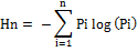 …...............(1) …...............(1)
Where, Pi is the proportion of built-up in the ith concentric circle. As per Shannon’s Entropy, if the distribution is maximally concentrated in one circle, the lowest value zero will be obtained.
- Computation of spatial metrics: Spatial metrics are helpful to quantify spatial characteristics of the landscape. These metrics quantify specific spatial characteristics of patches, classes of patches, or entire landscape mosaics. Selected spatial metrics were used to anlayse and understand the urban dynamics, FRAGSTATS (McGarigal and Marks, 1995) was used to compute metrics at three levels: patch level, class level and landscape level. There are many quantitative measures of landscape composition that include the proportion of the landscape in each patch type, patch richness, patch evenness, and patch diversity. Table 4 below gives the list of metrics along with their description that were considered for the study.
Indicator |
Formula |
Description |
Class level Landscape metrics |
Number of patches (Built-up)(NP) |

ni =number of patches in the landscape of patch type i.
Range: NP≥ 1
|
NP is the number of patches of a corresponding patch type. |
Percentage of landscape (Built-up)
(PLAND) |
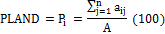
aij = area (m2) of patch ij.
A = total landscape area (m2).
Range: 0<PLAND≤ 100
|
PLAND is the percentage of landscape comprised of a corresponding patch type. |
Patch Density (PD) |
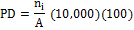
N =total number of patches in the landscape.
A =total landscape area (m2).
Range: PD> 0
|
PD is the number of urban patches divided by total landscape area. |
Normalised Landscape Shape Index
(NLSI) |
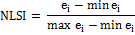
ei =total length of edge (or perimeter) of class i in terms of number of cell surfaces; includes all landscape boundary and background edge segments involving class i.
Range: 0 to 1
|
Normalized Landscape Shape Index is the normalized version of the landscape shape index (LSI) and provides a simple measure of class aggregation or Clumpiness. |
Area Weighted Mean Shape Index (AWMSI) |
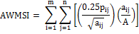
ai and pi are the area and perimeter of patch i, and N is the total number of patches.
Range: AWMSI >1, without limit.
|
It weighs patches according to their size; larger patches carry more weight than smaller ones.
It is also used to represent shape irregularities with small values indicating a regular shape and as the values increase, complexity and irregularities increase. |
Edge Density
(ED) |
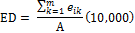
eik = total length (m) of edge in landscape involving patch type (class) i; includes landscape boundary and background segments involving patch type i.
A = total landscape area (m2). Range: ED > 0
|
ED standardizes edge on a per unit area basis that facilitates comparison between landscapes of different sizes. |
Clumpiness Index (Clumpy) |
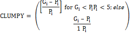
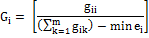
gii =number of like adjacencies (joins) between pixels of patch i based on the double-count method.
gik =number of adjacencies (joins) between pixels of patch types i and k based on the double-count method.
Min-ei = minimum perimeter (in number of cell surfaces) of patch type i for a maximally clumped class.
Pi =proportion of the landscape occupied by patch type i. Range: [-1,1]
|
Values of the clumpy index close to -1 is a measure of maximally disaggregated land use, whereas values of clumpy index close to 0 is indicative of distributed random patch and when clumpy index approaches 1, urban patch type is maximally aggregated.
|
Aggregation Index (AI) |
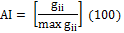
gii = number of like adjacencies (joins) between pixels of patch type i based on the single-count method.
max-gii = maximum number of like adjacencies (joins) between pixels of patch type i based on the single-count method.
|
AI equals 0 when the patch types have no like adjacencies. AI equals 100 when the landscape consists of a single patch. |
Interspersion & Juxtaposition Index
(Landscape level) (IJI) |
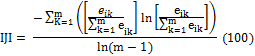
eik = total length (m) of edge in landscape between patch types I and k. m= number of patch type present in landscape.
Range: 0 < IJI ≤ 100
|
IJI approaches 0 when the corresponding patch type is adjacent to only 1 other patch type and the number of patch types increases. IJI = 100 when the corresponding patch type is equally adjacent to all other patch types |
Table 4: Landscape metrics calculated in the analysis
|