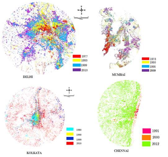
Temporal land use analyses reveal of a highly urbanized landscape and the influence of intense urbanisation in core areas on the buffer zones is evident with dispersed growth. Figure 4 illustrates the urban growth in Indian Mega cities during the past 4 decades. Figure 5 describes the land use details in each gradients during 1970 to 2010. All these cities experienced Infilling growth at the center, while post 1900, due to globalization these regions exhibit leap frog developments with dispersed growth at outskirts. The growth of urban pockets in these regions are circular and poly centric and in some locations axial growth depending of influencing agents. Kappa values calculated as part of accuracy assessment gave a median value of 0.85 for all cities considered, with overall accuracy of 89% on an average.

Figure 4. Change detection analysis representing the developments of urban footprint in various Megacities of India.

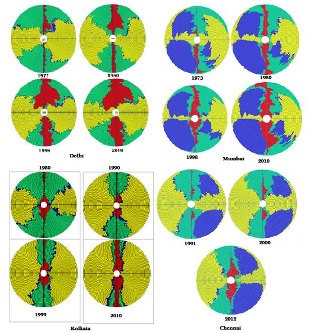
Figure 5. Representation of Gradient wise change land use distribution in 4 decades.

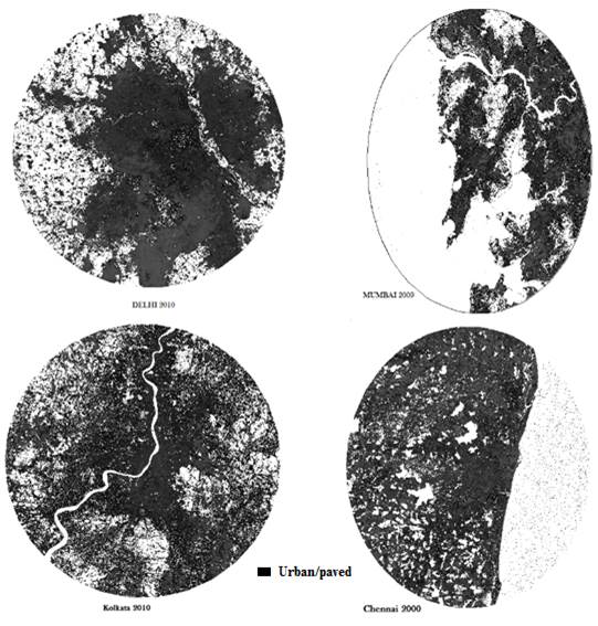
Spatial extent of urban built up computed through Normalised difference building index (NDBI) using temporal RS data are depicted in Figure 6. Comparison of NDBI with land use indicate the Kappa of 0.87 (for Delhi), 0.94 (Mumbai), 0.89 (Kolkata) and 0.88 (Chennai) respectively highlighting relatively accurate land use classification. Further the spatial patterns of urbanisation are assessed through computation of spatial metrics for gradients in four zones.

Figure 6. NDBI calculated for all Mega cities

6.1 Understanding the extent of urbanisation
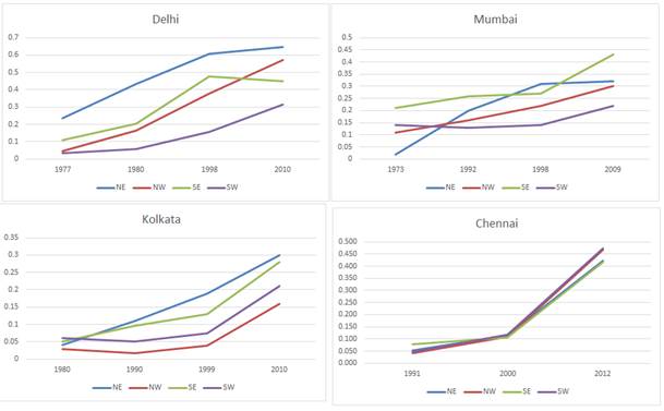
Shannon entropy was computed zone wise as a measure of extent of urbanisation. This helps in identifying the growth as concentrated or urban sprawl (Ramachandra et al., 2012b ; Ramachandra et al., 2013a; Bharath H. A. et al., 2012; Bharath s, et al., 2012). Higher the value of the Shannon entropy and closer to the threshold explains that the city is under the influence of sprawl. Lower the value indicates compact and monocentric urbanisation. Shannon entropy threshold values (log (n)) ranges from 1.49 (Delhi), 1.53 (Kolkata), 1.53 (Chennai) and 1.59 (Mumbai) Shannon entropy calculation for Delhi showed values reaching 0.7 in North east and North west direction, while Mumbai has a highest entropy values in South east and North east with a value reaching 0.45, Kolkata reaching the value of 0.35 in North east and South east in 2010, indicating that these cities experiencing tendency of sprawl and highlight the need for planning towards the provision of basic infrastructure.     

6.2 Spatial patterns of urbanisation through spatial metrics and PCA
Landscape metrics were calculated for each gradient of four zones in each city using Fragstat (Figure 7). To examine the overall spatial pattern variations in urban form across cities and over time, principal components analysis (PCA) was done. PCA helped in reducing the dimensionality while explaining variations in spatial data for pre 2000 and post 2000 (2009-12) of cities. This analysis helped in bringing out the similarities and differences between the gradients across cities

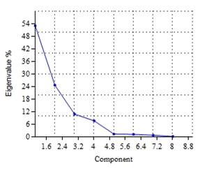
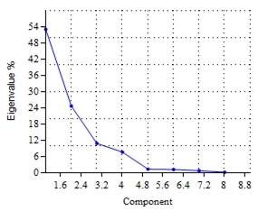
Scree plot pre-2000 and post 2000 of all 4 mega cities.is given in Figure 7 as shown below and based on variable representations by first three principal components with eigenvalues of over 1.5 were responsible for a total of 72% of the overall variance in all the metrics.

Figure 7. Shannon’s Entropy calculated for four Mega cities in India

Figure 8. Scree plot explaining the variability of respective components

Table 3 indicates that the first principal component is highly correlated with five variables -  Clumpy, LSI, LPI, IJI, NP and PD, which are measures of level of fragmentation in the landscape. Further this component suggests irregular shapes in the landscape due to higher patches with patch density. NP and PLAND with correlation of second component indicates large urban patches and higher percentage of urban land forms clusters and gradients. This component is negatively correlated with largest patches and percentage of urban land, which points to the fact that the percentage of urban land is less in these clusters.
Table 3. Correlation of metrics with principal components (pre 2000 data)

Biplot (Figure 9, corresponding to pre 2000) helped in understanding the directional gradient clusters that are formed representing same features in all four metros of India. Gradient clusters formed on extreme right are related with first principal component, of the buffer regions of all four metros which are very few in number. These areas are of very high fragmentation, complex shapes and less clumped (as these metrics are correlated with PCA1).

Further, the clusters located in the midway and closer to the axes correspond to comparatively less fragments (with near simple shapes) and these clusters are dominated by gradients of 1-13 corresponding to a central business district of all 4 metros, representing a compact growth.
Principal component 2 explains mainly the largest patches of urban domination and percentage of urban area in the landscape. Gradients in the top portion of plot are related to this component. Largest patches of urban area in found mainly in buffer zones of Delhi north east and North West. Less large patches of urban area and its dominance is found in the regions of North east of Mumbai, south east of Chennai and North West regions of Mumbai forming separate clusters based on the urban dominance. This analysis showed that these metros are clumped and are concentrated in CBD regions in 1990.

Figure 9. Biplot of principal components based on metrics of pre 2000

Post-2000: urbanisation pattern in four mega cities: As per Scree plot based on variable representations of principal components, first three components deemed useful in explaining the data.
Based on the correlation matrix, as in table 4, the first principal component is strongly correlated with 5 variables of Clumpy, LSI, LPI, NLSI, NP and PD suggesting that there are not much clumped growth, interspersion is less, and lower numbers of largest patches in the landscape. This in turn indicates that high values of patches with high patch density and more irregular shapes in the landscape. The first component strongly correlates with shape and increased patches and form gradient clusters representing irregular shape landscapes with high fragmented patched growth.

Table 4: Correlation of metrics with principal components (post 2000 data)

The second component strongly correlates with LPI and Pland, highlighting clusters and gradients represent large urban patches with higher percentage of urban land and negatively correlated with shapes and interspersion, which indicates more uniform shapes in these clusters and better interspersed. Third component doesn’t reveal any reasonable relationship among metrics.
Figure 10 is the plot of principal components which highlight the clustering of gradients with similar attributes in all 4 metros of India. Values on extreme right indicate that the clusters formed at extreme right mainly corresponds to gradients (correlated with PCA 1) of the buffer regions with very high fragmentation, complex shapes and less clumped of all four metros.

Further the clusters with comparatively less fragments with near simple shapes, are located in the midway and closer to the axes. Here the clusters indicate compactness and are dominated by gradients corresponding to circles 10-23, and few gradients of Chennai buffer zones.
Extreme left of Figure 10 shows least related values to the PCA 1 and are dominated by gradients from 1 to 12, corresponding to the regions with high clumped growth, simple shapes and least patches (to form single urban cluster).


Figure 10. Biplot of principle components based on metrics in 2009

Principal component 2 explains mainly the largest patches highlighting urban domination with higher percentage of urban area in the landscape. Largest urban patches are in buffer zones of Delhi north east and Chennai south east. Compared to this, relatively lesser urban patches and its dominance is found in north east of Mumbai, south east of Chennai and North West regions of Mumbai form separate clusters.

The gradients which are bordering buffer zones and the core area have also bigger urban patches and are comparatively smaller than urban patches in buffer zones. PCA thus aided in delineating highly fragmented urban patches in the buffer zones and highly clumped urban pockets near CBD (core area).