DATA AND METHODS

Data: Indian remote sensing (IRS) satellite data (Resourcesat 2, Cartosat 1) procured from the National Remote Sensing Centre, Hyderabad (http://nrsc.gov.in) were used in the analysis. The remote data was supplemented with datasets such as i) Survey of India topographic maps of 1:250,000, and 1: 50000 scale, ii) online data such as Google earth (http://earth.google.com), Bhuvan (http://bhuvan.nrsc.gov.in) and field data collected from wards using pre-calibrated GPS. These supplementary data sets were used for delineating and extracting administrative boundaries, geometrical correction of remote sensing data, classification, verification and validation of classified outputs. The GPS based field data along with the virtual online better spatial resolution remote sensing data were used for estimating number of trees per ward. Census of trees with canopy in select wards helped in assessing the tree distribution in each ward of Greater Bangalore. Table 2 gives the summary of the data used for inventorying and mapping of trees in Bangalore.

Table 2: Data used for inventorying and mapping trees in Bangalore

5.0 Method
To quantify ward-wise the number of trees per person in Bangalore, the protocol followed is given in Figure 2, which include i) Land use analysis using remote sensing, ii) land use changes using temporal remote sensing data, iii) deriving tree canopy, iv) canopy distribution in each ward, v) field data analysis – tree canopy distribution, vi) computation of number of trees in all wards based on field knowledge using remote sensing data, vii) computation of metrics (tree density, number of trees per person). 

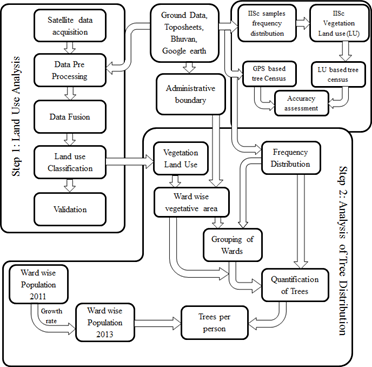
Figure 2: Method used for data analysis

Land use analysis using remote sensing data: The land use analysis of the acquired remote sensing data was carried out using the following steps: a) data pre-processing b) data fusion c) classification d) validation.

1. Temporal Land use analysis: The method involves i) generation of False Colour Composite (FCC) of remote sensing data (bands – green, red and NIR). This helped in locating heterogeneous patches in the landscape ii) selection of training polygons (these correspond to heterogeneous patches in FCC) covering 15% of the study area and uniformly distributed over the entire study area, iii) loading these training polygons co-ordinates into pre-calibrated GPS, vi) collection of the corresponding attribute data (land use types) for these polygons from the field. GPS helped in locating respective training polygons in the field, iv) supplementing this information with Google Earth v) 60% of the training data has been used for  classification, while the balance is used for validation or accuracy assessment. Land use analysis was carried out using supervised pattern classifier - Gaussian maximum likelihood algorithm. This has been proved superior classifier as it uses various classification decisions using probability and cost functions. Mean and covariance matrix are computed using estimate of maximum likelihood estimator (Ramachandra et al, 2013a; Ramachandra and Bharath, 2013; Vinay et al, 2012; Ramachandra et al., 2013b). Temporal remote sensing data was classified (described in table 3) into four categories: i) built up; ii) vegetation; iii) water; iv) others.

Table 3:  Land use categories

Land use Class	Land use included in class
Urban	Residential Area, Industrial Area, Paved surfaces, mixed pixels with built-up area
Water	Tanks, Lakes, Reservoirs, Drainages
Vegetation	Forest, Plantations
Others	Rocks, quarry pits, open ground at building sites, unpaved roads, Croplands, Nurseries, bare land

Accuracy assessment to evaluate the performance of classifiers, was done with the help of field data by testing the statistical significance of a difference, computation of kappa coefficients and proportion of correctly allocated cases.    Statistical assessment of classifier performance based on the performance of spectral classification considering reference pixels is done which include computation of kappa (κ) statistics and overall (producer's and user's) accuracies. The classification of the data has been completed using “GRASS” – Geographic Resource Analysis Support System (http://ces.iisc.ernet.in/grass) open source GIS software by considering four land use classes.

2. Resourcesat and Cartosat data Pre-processing: The multi spectral remote sensing data (Resourcesat 2) and Cartosat 1 were geometrically corrected using ground control points collected from topographic maps, virtual remote sensing data as well as using GPS. This involved rectification of horizontal shifts. Resourcesat data has spatial resolution of 5.8 m (with multi spectral resolutions) and Cartosat data resolution is 2.7m. Fusion of these data, helped in optimizing spatial and spectral resolutions, which aided in mapping the canopy of trees.
3. Data Fusion: Fusion of data from multiple sensors aids in delineating objects with comprehensive information due to the integration of spatial information present in the high resolution (HR) panchromatic (PAN) image and spectral information present in the low resolution (LR) Multispectral (MS) images.  Image fusion techniques integrate both PAN and MSS and can be performed at pixel levels. Data fusion (Resource sat and Cartosat data) was performed using algorithms - Hyperspectral Color Space resolution (HCS) merge, High Pass Filter (HPF) fusion, Modified Intensity Hue Saturation (MHIS) fusion, Wavelet Fusion.
4. Fused data Classification:  Fused remote sensing data was classified into four categories (table 3), all these four classes were combined to two land use classes i.e., Vegetation (Trees) and non-vegetation. The fused high resolution satellite images were classified using the Gaussian Maximum Likelihood Classifier (MLC) algorithm (Lillesand et al, 2004) to classify each pixel into a particular land use class. Fused data was classified using MLC with help of training data sets that were acquired from the field and supplementary data from Bhuvan and Google earth.
5. Validation: The validation of the classified land use image was completed though the accuracy assessment and kappa statistics, for measuring the level of agreement between the classified land use image and a reference land use image and to assess the performance of the classifier (Ramachandra et al., 2012a; Bharath et al., 2012; Ramachandra and Bharath, 2012).

Analysis of Tree Distribution: The analysis of tree distribution was carried out based on frequency distribution of the tree canopy area. The method involved in assessing the distribution includes: a) Data Collection, b) Frequency distribution analysis, c) Computation of tree distribution in each ward.

1. Data Collection: Trees with its canopy (spatial extent) were mapped in select wards (covering 10% of Bengaluru’s spatial extent) using pre-calibrated GPS. Tree canopy of these trees were also delineated using higher spatial resolution virtual data (Bhuvan, Google Earth). This gave information such as species wise canopy spatial extent and number of species in sampled wards.
2. Frequency distribution: Based on the field data, histogram (frequency distribution) of tree canopy were computed. Administrative wards were grouped based on number of tress as i) wards with > 500 trees and ii) < 500 trees. The number of trees in each ward is computed (based on the tree distribution in each of sampled wards).
3. Computation of metrics:  Metrics such as population density, tree density and number of trees per person in each ward was computed. Population for 2013 was estimated under each ward based on the decadal growth and population of 2011 9based on population census data of 2011) using equation 1.

P2013(i) = P2011(i)*(1+n*r(i))                                    …1
Where P2013(i) - Population of ward i for the year 2013
P2011(i) - Population of ward i for the year 2011
n - Number of decades = 0.2, r(i) – Incremental rate of ward i.
Number of trees per person in each ward is computed using equation 2.
TpP(i) =             ------2
Trees per person for Bangalore is computed by aggregating for all wards as in equation 3
TpP(B) =        ……..3
Where TpP(i)- Tree per person in ward i, Tree(i) - Number of trees in ward i.
TpP(B) - Tree per person in Bangalore

4. Validation:Trees extracted from remote sensing data (for each ward) was compared with the field data using equation 4.  Frequency distribution of canopy (based on size) was also compared with the field data.  Census of trees in Indian institute of Science campus (178 hectares spatial extent) was done using GPS.  Data collected from field include spatial location of a tree, size of its canopy, habit (tree/shrub/ climber/herb), species details. Canopy of these trees were also digitized using virtual data (Google Earth, Bhuvan). Frequency distribution of trees based on the canopy data was computed. Canopy mapping for the campus was done using fused remote sensing data (with spatial resolution of 2.7 m Cartosat and Multi spectral data (5.8 m spatial resolution) of Resourcesat). Canopy were grouped based on size and histogram was generated.

Accuracy = 100 – (abs ((ClassTree – GPSTree)/GPSTree) *100)                 ….4
Where ClassTree - Tree count based on classified data
GPSTree - Tree count based on field census using GPS