 |
GRASS with R: An Introductory Tutorial to Open Source GIS & Statistical Computing Software for Geospatial Analysis |
 |
1Energy and Wetlands Research Group, Centre for Ecological Sciences [CES], 2Department of Management Studies, 3Centre for Sustainable Technologies (astra),
4Centre for infrastructure, Sustainable Transportation and Urban Planning [CiSTUP],
Indian Institute of Science, Bangalore – 560012, India.
*Corresponding author: cestvr@ces.iisc.ac.in
|
SPATIAL ANALYSIS WITH R
The R spatial analysis packages include spatial point processing, spatial autocorrelation, smoothing, interpolation, geostatistics, etc. The “sp” package in R offers a wide variety of geostatistical functions such as foundation classes, interface to coordinate systems, utility plotting methods, sampling methods, etc. Other R geospatial packages are listed in Table II.
Table II: R Spatial Analysis Programs
| Sl.No. |
Package |
Purpose |
| 1 |
maptools |
reading and handling of shape files |
| 2 |
maps |
drawing of basic geographical maps |
| 3 |
spgpc |
polygon clipping |
| 4 |
spGDAL |
Geospatial Data Abstraction Library |
| 5 |
spatial |
spatial point pattern analysis |
| 6 |
spatstat |
2D point patterns multitype/marked points and spatial covariates, functions for exploratory data analysis, model-fitting, simulation, model diagnostics, and formal inference |
| 7 |
splancs |
space-time, emphasis on points-within-polygons |
| 8 |
spdep |
spatial regression, autocorrelation |
| 9 |
gstat |
univariate and multivariate geostatistics |
| 10 |
geoR |
model based geostatistics |
| 11 |
geoRglm |
inference in generalised linear spatial models |
| 12 |
fields |
curve and function fitting with an emphasis on splines, spatial data and spatial statistics, spatial covariance |
| 13 |
RArcInfo |
reading ArcInfo version 7 and e00 files |
| 14 |
shapefiles |
reading and writing ESRI shapefiles |
| 15 |
RColorBrewer |
color palettes optimized for thematic maps, etc. |
- R as a Calculator: R language use the usual arithmetic operators and the data type used is modes. The modes are logical, numeric and complex numbers. One of the simple possible tasks in R is to enter an arithmetic operation and receive a result. For example, if we want to add two numbers then we can type in the terminal
>2+2
>4
- Assigning value to variables: R has symbolic variables like any other programming language that is used to represent value to the assigned variable. The operator “<-” is known as assignment operator and it assigns the value of the expression on right to the object on left. For example, we can assign 5 to the variable x which can be used for subsequent arithmetic expression.
>x<-5
and then type
>x+x
to get 10 as our final output
- Methods of data entry: R can handle entire data vectors as single objects and there are various ways of inputting data in R. We can directly type the values in the command line with concatenation function “c”. Data can be entered one at a time from the keyboard using scan or “read.table” command.
w<- c(60, 72, 57, 90, 95, 72)
y <- scan( )
>data<-read.table(“read_my_file.txt”,header=T)
If the data is separated by “tab” or “space” then it can be specified in the command
>data<-read.table(“read_my_file.txt”,sep=“/t”,header=T)
>attach (data)
>names(data)
- Arithmetic operations: In R many complicated calculations can be done by using addition, substraction, multiplication, division and exponentiation as operator.
>x<-3+8
>5^2-5*2
[1] 15 will appear as the outcome. Its better to specify the order of evaluation of expression by using parenthesis and no space is required to separate components in an arithmetic operation.
>1-3*3
[1] -8
- Useful Builtin Function: Many calculations are already built into the program [2] and results can be easily obtained by using these functions as listed in Table III.
Table III: R built in functions.
| Sl. No. |
Function |
Purpose |
| 1 |
mean |
to find average |
| 2 |
sd |
to find standard deviation |
| 3 |
max |
to obtain maximum element in a data set |
| 4 |
min |
to find minimum element in a data set |
| 5 |
range |
to find range of values |
| 6 |
median |
to find median of the data set |
| 7 |
var |
to find variance of the data set |
| 8 |
sort |
command for sorting in increasing order of magnitude |
| 9 |
diff |
creates a vector of differences by substracting previous element from next element. |
| 10 |
cov(a,b) |
covariance between a and b |
| 11 |
cor(a,b) |
correlation between a and b |
| 12 |
length(a) |
length of a vector |
| 13 |
floor(x) |
round down to next lowest integer |
| 14 |
ceil(x) |
round up next largest integer |
| 15 |
round(x) |
round to nearest integer |
| 16 |
anova |
analysis of variance |
| 17 |
summary (x) |
summarises the data (x) |
| 18 |
assign(“x”,3) |
assigns the value 3 to object x |
| 19 |
c() |
combines or concatenates terms together |
| 20 |
rep(x, each=4) |
repeats x 4 times |
- Graphics with R: R provides flexible and powerful graphical analysis. There are a number of commands which helps in obtaining simple graphs through R by using the command “plot” and giving various specifications about the appearance of the graph in both x and y axis. Table IV lists some of the standard plot functions.
A simple example is to plot a sine curve. First the intervals are defined along with the number of data points to support the curve.
>x <- seq(-2*pi, 2*pi, len = 100)
>x
>str(x)
>summary(x)
Then we can plot it (the type parameter specifies the line type):
matplot(x, sin(x), type=“l”)
To get an idea about the various “matplot()” options, run:
>?matplot
You can see some “matplot()” examples by running:
>example(matplot)
More examples follows:
>barplot(table(x),xlab=“DigitalNumbers”,ylab=“Frequency”,col“gray70”); where x is the data which is already being inputed in R
> plot(c,xlab=“BANDS”,ylab=“Digital Number”)
> boxplot(a,xlab=“BANDS”,ylab=“Digital Number) where a is the data set which R statistical software has already read.
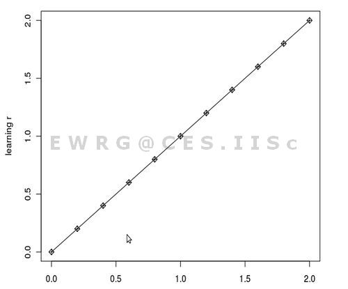
Figure 1: Line graph generated in R.
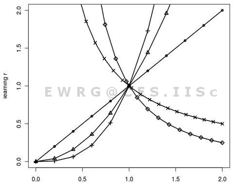
Figure 2: Quadratic line graph obtained in R
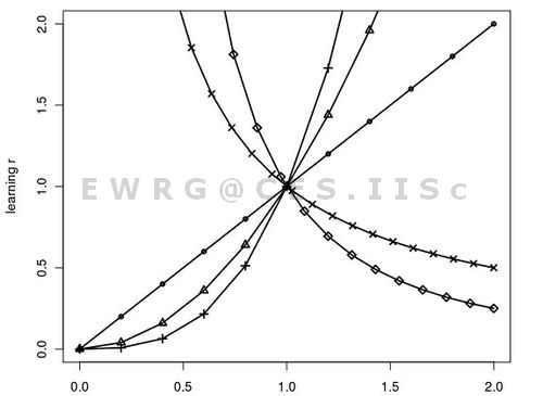
Figure 3: Line with quadratic, cubic, power -1 and power -2 generated in R
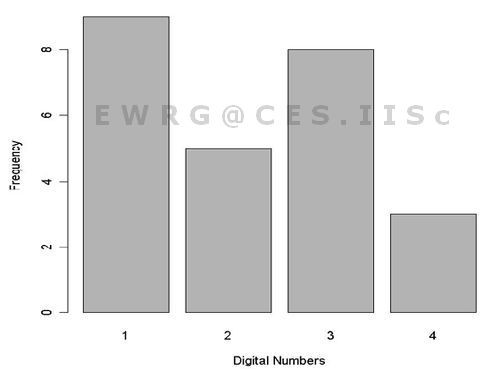
Figure 4: Bar plot
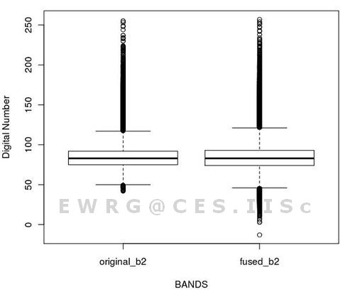
Figure 5: Boxplot
Table IV: Standardr plot functions
| Sl. No. |
Function |
Name of the plot |
| 1 |
plot() |
Scatterplot |
| 2 |
hist() |
Histogram |
| 3 |
boxplot() |
Box-and-whiskers plot |
| 4 |
stripchart() |
Stripchart |
| 5 |
barplot() |
Bar diagram |
| 6 |
stem() |
Stem-and-leaf display |
- Saving, Storing and Retrieving Work in R: When we quit R session, we should tupe “yes” to “save workspace image”. When we restart R all the data and variables from the previous session are available.
- Getting help in R: To get help in R use “help.search” function with the query in double quotes “ ”, for example help.search “data input ”.
- Add-on (CRAN) Packages in R: R has numerous addon packages for different applications. Packages can be downloaded for the CRAN Mirror site (http://cran.r-project.org/) and installed in R. Table V prensents some of the R packages. More packages can be found on http://cran.r-project.org/. If we want to install packages then the simple command is “install.packages” or from the Linux Terminal type: $R CMD INSTALL package_name.tar.gz. For example, “R CMD INSTALL spgrass6 _0.3-7.tar.gz”.
Table V: Standard packages in R.
| Sl. No. |
Package |
Purpose |
| 1 |
nortest |
Normality test |
| 2 |
randomforest |
Classifier |
| 3 |
cluster |
Clustering tool |
| 4 |
rgdal |
Geospatial abstraction data library in R |
| 5 |
raster |
Geographic analysis and modelling with raster data |
| 6 |
kohonen |
Supervised and unsupervised self-organising maps |
| 7 |
tseries |
Time-series data analysis |
|
|
Citation : Anindita Dasgupta, Uttam Kumar, Chiranjit Mukhopadhyay and Ramachandra. T.V., 2012, GRASS with R: An Introductory Tutorial to Open Source GIS & Statistical Computing Software for Geospatial Analysis, Proceedings of the OSGEO-India: FOSS4G 2012- First National Conference "OPEN SOURCE GEOSPATIAL RESOURCES TO SPEARHEAD DEVELOPMENT AND GROWTH”, 25-27th October 2012, @ IIIT Hyderabad , pp. 1-6.
|