|
RESULTS AND DISCUSSION
1. Fusion of 1:4 resolution ratio (IRS PAN 5.8 m + LISS-III MS 23.5 m)
The five image fusion techniques were applied on IRS PAN and LISS-III MS bands (Table 1) as shown in Figure 2. A 5 x 5 filter was used in SFIM, HP Fusion, HP Filter and HPM. A linear regression of IRS PAN and LISS-III MS sensor Spectral Response Function (SRF) (values were obtained from Space Application Centre (SAC), Ahmedabad, India) is carried out (Figure 1). The regression coefficient  is derived for each MS band. ( is derived for each MS band. ( , , and and  ) for IRS-1D LISS-III MS 3 bands. ) for IRS-1D LISS-III MS 3 bands.
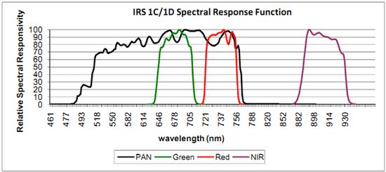
Figure 1: Spectral response pattern of IRS 1C/1D PAN and LISS-III MS bands.
 and and  for IRS 1D is ( for IRS 1D is ( , ,  , and , and  ). ).
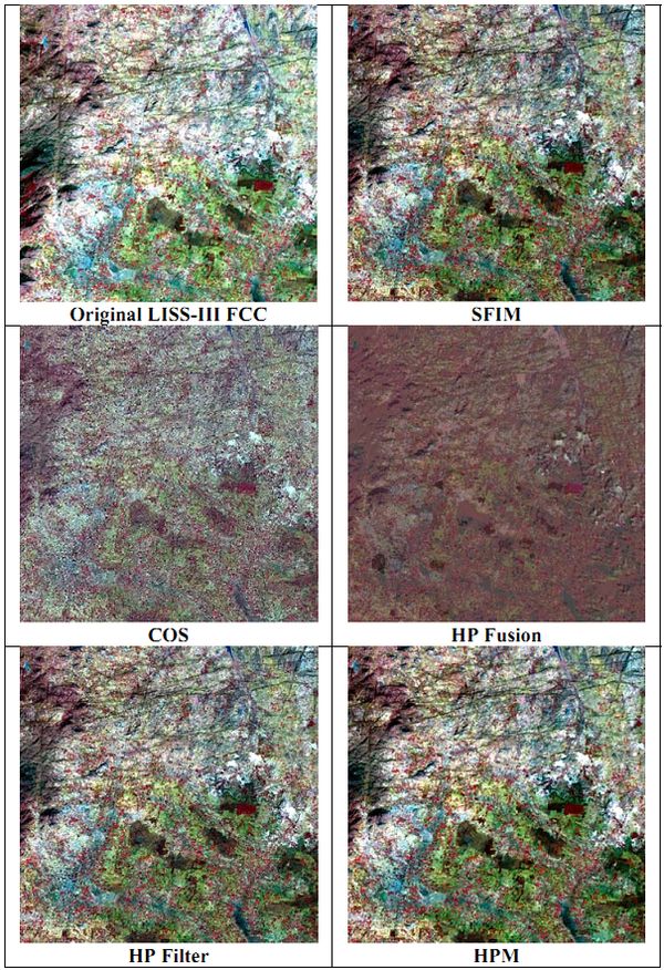
Figure 2: IRS LISS-III MS + PAN fused outputs at 6 m from 5 best performing techniques
It is apparent from Figure 2 that SFIM, HP Filter and HPM have produced good quality images. COS, and especially HP Fusion have produced significant colour distortion. The UIQI values, CC of PAN with synthetic PAN, and CC between original and degraded fused images closest to 1 and min, max, and sd values closer to original band values are highlighted in Table 2, 3 and 4.
Table 2: UIQI measurements of the similarities between original IRS LISS-III MS and fused bands and correlation between IRS PAN and simulated PAN
| Sl. No. |
Algorithms |
Green |
Red |
NIR |
CC (p value < 2.2e-16) |
| 1 |
SFIM |
0.95 |
0.97 |
0.93 |
- |
| 2 |
COS |
0.03 |
0.05 |
0.01 |
1 |
| 3 |
HP Fusion |
0.61 |
0.65 |
0.61 |
-0.92 |
| 4 |
HP Filter |
0.88 |
0.92 |
0.85 |
0.95 |
| 5 |
HPM |
0.99 |
0.99 |
0.99 |
0.95 |
Table 3: Minimum and maximum values of the IRS LISS-III MS original and fused bands
| Sl. No. |
Algorithms |
Minimum |
Maximum |
| |
|
Green |
Red |
NIR |
Green |
Red |
NIR |
| |
Original bands |
42 |
28 |
26 |
252 |
247 |
187 |
| 1 |
SFIM |
35 |
26 |
25 |
261 |
247 |
195 |
| 2 |
COS |
-217 |
-215 |
-285 |
465 |
456 |
512 |
| 3 |
HP Fusion |
-4.8 |
-19.8 |
-14.6 |
174 |
167 |
135 |
| 4 |
HP Filter |
-13 |
-17 |
-1 |
257 |
244 |
194 |
| 5 |
HPM |
42 |
28 |
26 |
264 |
256 |
197 |
Table 4: Standard deviation and correlation values between the IRS LISS-III MS original and fused bands
| Sl. No. |
Algorithms |
Standard deviation |
CC (p value < 2.2e-16) |
| |
|
Green |
Red |
NIR |
Green |
Red |
NIR |
| |
Original bands |
13 |
17 |
12 |
- |
- |
- |
| 1 |
SFIM |
14 |
17 |
13 |
0.95 |
0.97 |
0.93 |
| 2 |
COS |
88 |
87 |
109 |
0.34 |
0.37 |
0.29 |
| 3 |
HP Fusion |
11 |
13 |
10 |
0.82 |
0.88 |
0.78 |
| 4 |
HP Filter |
15 |
18 |
14 |
0.88 |
0.92 |
0.85 |
| 5 |
HPM |
13 |
17 |
12 |
0.99 |
0.99 |
0.99 |
From the above fusion quality measures, it is evident that HPM retained most of the statistical properties of IRS LISS-III MS fused bands and is most suitable technique for merging IRS MS and PAN images.
2. Fusion of 1:2 resolution ratio (Landsat ETM + PAN 15 m + MS 30 m)
Linear regression of Landsat ETM+ PAN and MS sensor SRF (http://landsathandbook.gsfc.nasa.gov/handbook/handbook_htmls/chapter8/chapter8.html) is shown in Figure 3. Regression coefficient are  , ,  , ,  , ,  , ,  and and  for MS 6 bands (except band 6 - thermal band); for MS 6 bands (except band 6 - thermal band);  ; ;  is ( is ( , ,  , ,  , ,  , ,  and and  ). ).
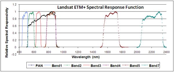
Figure 3: Spectral response pattern of Landsat ETM+.
The five image fusion techniques were applied on Landsat ETM+ PAN and MS bands as shown in Figure 4. Statistical properties of the fused images were assessed as per Table 5-9.
Table 5: UIQI measurements of the similarities between Landsat ETM+ original and the fused bands and correlation between Landsat ETM+ original and simulated PAN
| Sl. No. |
Algorithms |
Blue |
Green |
Red |
NIR |
MIR-1 |
MIR-2 |
CC (p value = 2.2e-16) |
| 1 |
SFIM |
0.6756 |
0.8183 |
0.9136 |
0.8868 |
0.9280 |
0.9373 |
- |
| 2 |
COS |
0.99 |
0.99 |
0.99 |
0.99 |
0.98 |
0.98 |
1 |
| 3 |
HP Fusion |
0.5764 |
0.6349 |
0.7405 |
0.6873 |
0.8003 |
0.7600 |
0.34 |
| 4 |
HP Filter |
0.8334 |
0.8900 |
0.9595 |
0.8971 |
0.9755 |
0.9990 |
0.76 |
| 5 |
HPM |
0.75 |
0.84 |
0.93 |
0.90 |
0.96 |
0.95 |
0.76 |
Table 6: Minimum values of the Landsat ETM+ MS original and fused bands (1:2)
| Sl. No. |
Algorithms |
Minimum |
| |
|
Blue |
Green |
Red |
NIR |
MIR-1 |
MIR-2 |
| |
Original bands |
57 |
40 |
27 |
27 |
31 |
14 |
| 1 |
SFIM |
32 |
25 |
20 |
16 |
17 |
12 |
| 2 |
COS |
54 |
38 |
21 |
22 |
14 |
1 |
| 3 |
HP Fusion |
39 |
26 |
19 |
17 |
27 |
9 |
| 4 |
HP Filter |
42 |
25 |
18 |
14 |
18 |
8 |
| 5 |
HPM |
39 |
25 |
27 |
22 |
28 |
14 |
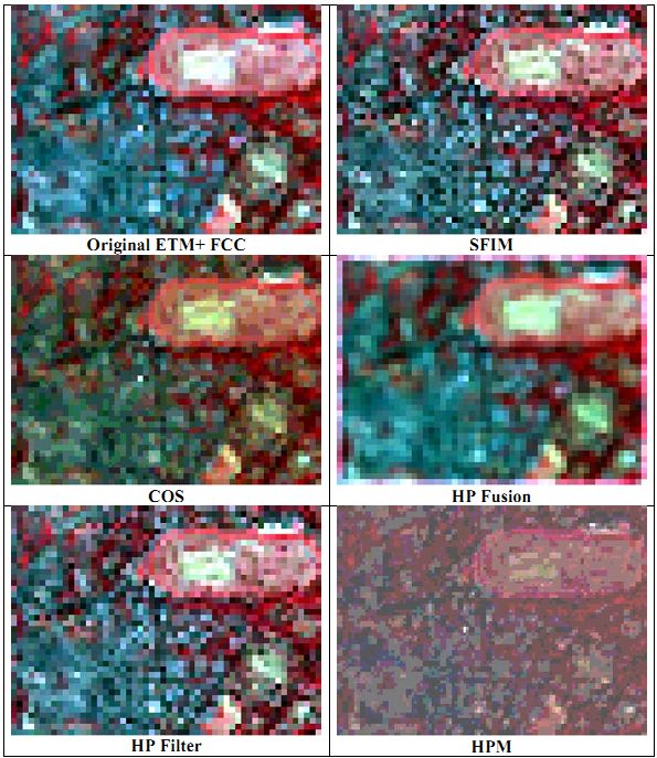
Figure 4: Landsat ETM+ PAN + MS fused outputs at 15m from 5 best performing techniques.
Table 7: Maximum values of the Landsat ETM+ MS original and fused bands (1:2)
| Sl. No. |
Algorithms |
Maximum |
| |
|
Blue |
Green |
Red |
NIR |
MIR-1 |
MIR-2 |
| |
Original bands |
144 |
139 |
168 |
102 |
233 |
200 |
| 1 |
SFIM |
305 |
290 |
349 |
184 |
372 |
381 |
| 2 |
COS |
154 |
146 |
179 |
105 |
269 |
227 |
| 3 |
HP Fusion |
88 |
81 |
108 |
82 |
143 |
121 |
| 4 |
HP Filter |
152 |
145 |
186 |
115 |
237 |
203 |
| 5 |
HPM |
167 |
160 |
242 |
127 |
272 |
238 |
Table 8: Standard deviation of the Landsat ETM+ MS original and fused bands (1:2)
| Sl. No. |
Algorithms |
Standard deviation |
| |
|
Blue |
Green |
Red |
NIR |
MIR-1 |
MIR-2 |
| |
Original bands |
10 |
13 |
22 |
14 |
29 |
26 |
| 1 |
SFIM |
15 |
17 |
26 |
16 |
32 |
29 |
| 2 |
COS |
11 |
14 |
25 |
14 |
36 |
32 |
| 3 |
HP Fusion |
8 |
9 |
15 |
10 |
20 |
17 |
| 4 |
HP Filter |
13 |
15 |
24 |
15 |
30 |
28 |
| 5 |
HPM |
15 |
17 |
26 |
16 |
33 |
29 |
Table 9: Correlation values between the Landsat ETM+ MS original and fused bands (1:2)
| Sl. No. |
Algorithms |
CC (p value < 2.2e-16) |
| |
|
Blue |
Green |
Red |
NIR |
MIR-1 |
MIR-2 |
| 1 |
SFIM |
0.73 |
0.84 |
0.92 |
0.90 |
0.93 |
0.94 |
| 2 |
COS |
0.99 |
0.99 |
0.99 |
0.99 |
0.99 |
0.99 |
| 3 |
HP Fusion |
0.63 |
0.73 |
0.87 |
0.79 |
0.92 |
0.89 |
| 4 |
HP Filter |
0.85 |
0.90 |
0.96 |
0.90 |
0.98 |
1.00 |
| 5 |
HPM |
0.80 |
0.87 |
0.94 |
0.91 |
0.94 |
0.95 |
From the fusion quality assessment it is apparent that HPM has significantly distorted the colour. COS is best for fusing 1:2 Landsat ETM+ PAN and MS bands. A reason for better performance of COS than others could be the well defined spectral response function of Landsat ETM+, where the wavelength of PAN band (0.520-0.900 μm) completely encompasses the VIS (visible - G, R) and NIR bands (0.525-0.900 μm). Note that in case of IRS sensor, PAN wavelength only encompasses the G and R bands, and so the same technique could not perform well.
3. Fusion of 1:50 resolution ratio (IRS PAN 5 m + MODIS 250 m)
The five image fusion techniques were applied on IRS PAN at 5 m and MODIS 7 bands at 250 m. SRF of IRS 1C/1D PAN and MODIS 7 bands is shown in Figure 5.
 , ,  , ,  , ,  , ,  , ,  and and  ; ;  ; ;  is ( is ( , ,  , ,  , ,  , ,  , ,  and and  ). ).
The original, fused images and statistical properties of the fused bands (not shown here due to space constraint) reveal that while HPM has significantly distorted the colour. HP Filter followed by HP Fusion and HPM perform best on the fusion of 1:50 resolution ratio. It is to be noted that the filtering techniques have performed better here, than COS. One reason for poor performance of COS is that, IRS PAN sensor wavelength only encompasses MODIS band 3 (B) and 4 (G) part of the EM spectrum (see Figure 5). Since all other MODIS bands do not intersect with the IRS PAN band in the corresponding wavelength region, so the fusion quality of COS has degraded. It is to be noted that these fused images are not very useful for visual assessment of the results.
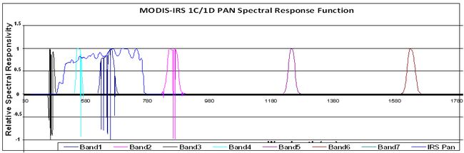
Figure 5: Spectral response pattern of IRS 1C/1D PAN-MODIS.
4. Fusion of 1:100 resolution ratio (IRS PAN 5 m + MODIS 500 m)
SRF of IRS 1C/1D PAN and MODIS 7 bands are same as Figure 5.  , r and , r and  are same as in 1:50 resolution ratio (IRS PAN + MODIS 250 m). The original, fused images and statistical properties of the fused bands (not shown here) reveal that SFIM has abrupt change in digital numbers while HPM has greatly distorted the colour in the fused image. HP Filter produced fused images that are closest to the original images. are same as in 1:50 resolution ratio (IRS PAN + MODIS 250 m). The original, fused images and statistical properties of the fused bands (not shown here) reveal that SFIM has abrupt change in digital numbers while HPM has greatly distorted the colour in the fused image. HP Filter produced fused images that are closest to the original images.
5. Fusion of 1:250 resolution ratio (IKONOS PAN 1 m + MODIS 250 m)
SRF of MODIS 7 bands are as shown in Figure 6.
 , ,  , ,  , ,  , ,  , ,  and and  ; ;  ; ;  for IKONOS is ( for IKONOS is ( , ,  , ,  , ,  , ,  , ,  and and  ). ).
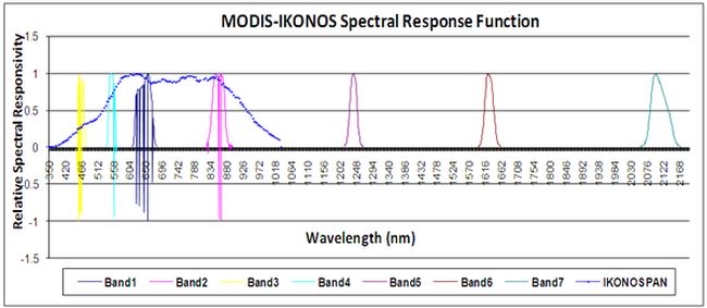
Figure 6: Spectral response pattern of MODIS-IKONOS.
Figure 6 shows that IKONOS PAN band encompasses only MODIS band 1-4 (B, G, R and NIR). Visual appearance of fused images (not shown here) does not bring any sharpness and one may not see significant improvement in the pixel’s appearance before and after image fusion. However, statistical properties of the fused images reveal that HP Filter retains all the properties after fusion.
6. Fusion of 1:500 resolution ratio (IKONOS PAN 1 m + MODIS 500 m)
SRF of MODIS 7 bands and IKONOS PAN are same as Figure 6.  , r and , r and  are also same as in 1:250 resolution ratio (IKONOS PAN + MODIS 250 m). Although statistical measures reveal that HP Filter is most successful in retaining statistical properties of the original bands, advantages of image fusion with ratio 1:500 are not evident from the fused images. Table 10 summarises the best technique for each resolution ratio. Visual fusion qualities in Table 10 are graded as bad, good and excellent depending upon how clearly the objects could be identified, amount of colour distortion and sharpness of boundaries of objects in the fused images. are also same as in 1:250 resolution ratio (IKONOS PAN + MODIS 250 m). Although statistical measures reveal that HP Filter is most successful in retaining statistical properties of the original bands, advantages of image fusion with ratio 1:500 are not evident from the fused images. Table 10 summarises the best technique for each resolution ratio. Visual fusion qualities in Table 10 are graded as bad, good and excellent depending upon how clearly the objects could be identified, amount of colour distortion and sharpness of boundaries of objects in the fused images.
Table 10: Optimum fusion technique for various resolution ratios and sensors
| Sl. No. |
Resolution ratio |
Data |
Resolution in m |
Technique |
Visual fusion quality |
| 1 |
1:4 |
IKONOS PAN and MS |
1 m + 4 m |
SFIM |
Excellent |
| 2 |
1:4 |
IRS PAN and LISS-III MS |
6 m + 24 m |
HPM |
Excellent |
| 3 |
1:2 |
Landsat PAN and MS |
15 m + 30 m |
COS |
Excellent |
| 4 |
1:50 |
IRS PAN and MODIS |
5 m + 250 m |
HP Filter |
Good |
| 5 |
1:100 |
IRS PAN and MODIS |
5 m + 500 m |
HP Filter |
Good |
| 6 |
1:250 |
IKONOS PAN and MODIS |
1 m + 250 m |
HP Filter |
Bad |
| 7 |
1:500 |
IKONOS PAN and MODIS |
1 m + 500 m |
HP Filter |
Bad |
From the above study, it may be concluded that fusion of high and moderate spatial resolution MS band with HSR PAN band retains the spatial and spectral properties of the fused bands. However, as the spatial resolution decreases, fusion of images does not facilitate image quality enhancement for object identification. The fusion of multi-sensor data is limited by several factors. Often, lack of simultaneously acquired multi-sensor data hinders successful implementation of image fusion. In case of large differences in spatial resolution of input data, problems arise from limited (spatial) compatibility. Since there is no standard procedure of selecting the optimal data set, the user is often forced to work empirically to find the best result.
The fusion techniques are very sensitive to mis-registration. In some cases, especially if images of different spatial resolutions are involved, resampling of low resolution image to the pixel size of high resolution image might cause a blocky appearance. Therefore a smoothing filter can be applied before actually fusing the images (Chavez, 1991). The resulting image map can be further evaluated and interpreted related to the desired application.
Once the fused images were obtained, pattern classifiers were used to do the temporal analysis of the status of wetlands in Greater Bangalore as shown in Table 11 and Figure 7. The analyses indicate the decline of 34.48% during 1973 to 1992, 56.90% during 1973-2002 and 70.69% during 1973-2007 in the erstwhile Bangalore city limits. Similar analyses done for Greater Bangalore (i.e. Bangalore city with surrounding 8 unicipalities) indicate the decline of 32.47% during 1973 to 1992, 53.76% during 1973-2002 and 60.83% during 1973-2007.
Table 11: Status of wetlands in Bangalore city limits and Greater Bangalore
| |
Bangalore City |
Greater Bangalore |
| |
Number of
Wetlands |
Area (in ha) |
Number of
Wetlands |
Area (in ha) |
| SOI |
58 |
406 |
207 |
2342 |
| 1973 |
51 |
321 |
159 |
2003 |
| 1992 |
38 |
207 |
147 |
1582 |
| 2002 |
25 |
135 |
107 |
1083 |
| 2007 |
17 |
87 |
93 |
918 |
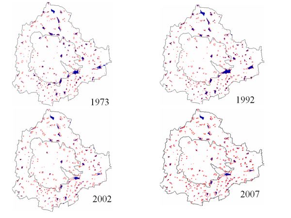
Figure 6: Spatio-temporal analysis of wetlands of Greater Bangalore. Wetlands are represented in blue and the vector layer of wetlands generated from SOI Toposheet is overlaid in red. The inner boundary (in black) is the Bangalore city limits and the outer boundary represents the spatial extent of Greater Bangalore.
There were 159 wetlands spread in an area of 2003 ha in 1973, that number declined to 147 (1582 ha) in 1992, which further declined to 107 (1083 ha) in 2002, and finally there are only 93 wetlands (both small and medium size) with an area of 918 ha in Greater Bangalore region in 2007. Wetlands in the northern part of Greater Bangalore are in a considerably poor state compared to the wetlands in southern Greater Bangalore. Validation of these wetlands were done through field visits during July 2007, which indicate an accuracy of 91%. The error of omission was mainly due to the cover of water hyacinth (aquatic macrophytes) in wetlands due to which the energy was reflected in IR bands rather than getting absorbed. Fifty-four wetlands were sampled through field visits while the remaining wetlands were verified using online Google Earth (http://earth.google.com).
Disappearance of wetlands and a sharp decline in the number of wetlands in Bangalore is mainly due to intense urbanization and urban sprawl. Many lakes were encroached for illegal buildings (54%). Urbanisation and the consequent loss of lakes has led to decrease in catchment yield, water storage capacity, wetland area, number of migratory birds, floral and faunal diversity and ground water table. Studies reveal the decrease in depth of the ground water table from 10-12 m to 100-200 m in 20 years due to the disappearance of wetlands. Field surveys (during July-August 2007) show that nearly 66% of lakes are sewage fed, 14% surrounded by slums and 72% showed loss of catchment area. Also, lake catchments were used as dumping yards for either municipal solid waste or building debris. The areas surrounding these lakes have illegal constructions of buildings and most of the time slum dwellers occupy the adjoining areas. At many sites, water is used for washing and household activities and even fishing was observed at one of these sites. Multi-storied buildings have come up on some lake beds that have totally intervened with the natural catchment flow leading to a sharp decline in the catchment yield and also a deteriorating quality of wetlands. Some of the lakes have been restored by the city corporation and the concerned authorities in recent times. These lakes have a well defined boundary, clean water and are maintained by the neighborhood people. These lakes are used for recreational purposes. They are home to migratory birds and also add aesthetic beauty to the surroundings.
|
