| Previous Session | Paper 1 | Next Session |
SESSION-9
PAPER-1: Numerical simulation of circulation in the chilika lake
G. Jayaraman, A. D. Rao, A. Dube and P. K. Mohanty
CONTENTS-
Abstract
Introduction
Hydrodynamic Model
Results and Discussion
Acknowledgements
References
| Abstract | up | previous | next | last |
Chilika Lake, (190 28' N - 190 54 ' N; 850 06' E - 850 36') on the Orissa coast, India, is one of the unique ecospheres in the world. It is the largest brackish water lagoon with estuarine character. On account of its rich biodiversity and socio economic importance, it is designated as a Ramasar site'- a wetland of international importance. Based on the circulation / hydrodynamics of the lake, the lake is divided into four sectors. The northern sector receives discharges of the floodwaters from the tributaries of the river Mahanadi. The southern sector is relatively smaller and does not show much seasonal variation in salinity. The central sector has features intermediate of the other sectors. The eastern sector, which is a narrow and constricted outer channel, connects the lagoon with the Bay of Bengal and the tidal effects are important in that area. Thus, due to its complicated geomorphology, the circulation in the lake corresponding to the different sectors is very complex. Interest in detailed analysis of the circulation, biotic and abiotic factors affecting the lake and its limnology is due to the threat to the lake from various factors Eutrophication, weed proliferation, siltation, industrial pollution and depletion of bioresources. The present paper deals with the numerical simulation of seasonal circulation in the lake. The theoretical formulation leads to a vertically integrated non-linear model, which includes the effects of wind in two different seasons on the circulation of the lake. In addition, the effect of the complicated boundary as well as the different type of circulation in different sectors of the lake is evaluated. The model is capable of accurate simulation of tidal elevations throughout the lake. A physico - biological model that incorporates the present dynamical model can be used to study the distribution of nutrients and chlorophyll in the lake.
| 1. Introduction | up | previous | next | last |
Wetlands play a central role in regional hydrologic and biogeochemical cycles, in maintaining biodiversity and in a wide range of human activities. Over the past two centuries, industrialization, urbanization and deforestation have led to the wetland loss resulting in the extinction of countless species and alteration of the relationship of wetlands with the regional environment. The physical processes in large lakes are complicated due to the flow regime, effluent discharge from urban runoffs and treated/untreated pollution sources.
The present study is concerned with the seasonal circulation in the Chilika lagoon the largest brackish water lagoon in India situated along the East Coast in the state of Orissa. The interest and thrust in studying the ecology of the lake is due to the increasing threat to the lake in the form if siltation, choking of the mouth and outer channel, eutrophication, weed infestation, salinity changes and decrease in fishery resources. Description of our study area and its present status are given in detail in our companion paper (Mohanty et al, 2002) and we shall not go into those here. A comprehensive multidisciplinary approach based on modeling and observational studies is required to formulate realistic strategy towards protection and conservation of the lake. In the current study, we examine the basic physical processes in the lake controlled by seasonal variations. The objective is to prepare ground for formulating a physico biological model to understand the seasonal cycle of the plankton productivity in the lake. The current profile developed in this model will be fitted into the biological model to study how the physical transport processes affect (i) the feeding or predator prey interaction and (ii) carry passive organisms eggs and larvae into areas that are safer for survival. A brief introduction to the hydrology and the hydrodynamic model for the lake is given in section 2. Section 3 describes the grid generation for the numerical scheme used to handle the complicated chilka topography. It also includes the results and discussions related to the seasonal circulation in the lake.
| 2. Hydrodynamic Model | up | previous | next | last |
2.1 Hydrology of the lake
The water spread area of the Chilika lake varies between 1165 to 906 sq km during the monsoon and summer respectively. A significant part of the fresh water and silt input to the lake comes from Mahanadi and its distributaries. Direct rainfall on the lake surface also makes a significant contribution to the fresh water input to Chilika. The lake shows an overall increase in depth of about 50 cm 1 m due to monsoon. The mouth connecting the channel to the sea is close to the northeastern end of the lake. High tides near the inlet mouth drive in salt water through the channel during the dry months, from December to June. The lake area proper experiences mean wind' speeds ranging from 5 kmph in winter to 10 15 kmph in summer. The coastal areas experience higher average wind speeds up to 25 kmph. (Nayak et al, 1998; Chandramohan et al, 1998)
It is important to study the seasonal circulation in the lake since the cyclic variation is key to maintaining the high biodiversity of the area. A distinct salinity gradient exists along the lagoon due to the influx of fresh water during monsoon and due to the inflow of seawater through the outer channel. This periodicity is responsible for maintaining the different species marine, estuarine and fresh water ones. Also, the currents regulate the supply of dissolved inorganic nutrients to the surface layer where most of the phytoplanktons are found. They also control the light levels experienced by phytoplankton below the surface layer. Thus physical exchange process plays a key role in the sustainability of the planktonic food web.
Simulation of lagoon/estuarine processes may require detailed treatment of irregular boundaries, complicated bottom topography, tidal effects, sediment transport, chemical transformation, biological production etc. Knowledge of the circulatory dynamics of the lake in general and seasonal circulation in particular is a prerequisite to estimate the other events in the lake. For shallow lakes it is appropriate to average all physical variables over the depth. Equations describing the physical limnology are based on the hydrostatic equations of motion and Boussinesq approximation and are known as the shallow water equations. (Hutter et al, 1984)
2.2 Model simulation
For the formulation of the model, we use a system of rectangular Cartesian co-ordinates in which the origin O, is within the equilibrium level of the sea-surface, Ox points towards the east, Oy points towards the north and Oz is directed vertically upwards. In the formulation, the sphericity of the earth's surface is ignored, the displaced position of the free surface is given by ![]() and the position of the sea floor by
and the position of the sea floor by ![]() The basic hydrodynamic equations of continuity and momentum for the dynamical processes in the water body are given by
The basic hydrodynamic equations of continuity and momentum for the dynamical processes in the water body are given by
![]() --------------- (1)
--------------- (1)
![]() -------------------(4)
-------------------(4)
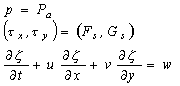
where ( ![]() ) are the Reynolds averaged components of velocity in the direction of
) are the Reynolds averaged components of velocity in the direction of ![]() respectively.
respectively. ![]() is the Coriolis parameter, g is the acceleration due to gravity, r is the density of the water supposed to be homogeneous and incompressible,
is the Coriolis parameter, g is the acceleration due to gravity, r is the density of the water supposed to be homogeneous and incompressible, ![]() are the x, y components respectively of the frictional surface stress, p is the pressure and t is the time. Molecular viscosity has been neglected. The terms in
are the x, y components respectively of the frictional surface stress, p is the pressure and t is the time. Molecular viscosity has been neglected. The terms in ![]() are included to model vertical turbulent diffusion. Denoting the wind stress and bottom stress components as
are included to model vertical turbulent diffusion. Denoting the wind stress and bottom stress components as ![]() and
and ![]() respectively and the surface pressure as
respectively and the surface pressure as ![]() , the boundary conditions become
, the boundary conditions become
![]()
![]() --------------------(6)
--------------------(6)
The last condition is the kinematic surface condition and expresses the fact that the free surface is materially following the fluid. Since the main objective lies in the prediction of long waves in shallow coastal waters, it is reasonable to assume that the wavelength is large compared to the depth. With this assumption, it may be shown that equation (4) reduces to hydrostatic pressure approximation
![]() --------------------------------(7)
--------------------------------(7)
The principal equations (1), (2), (3), and (7) could be solved, but the procedure would be laborious because of the presence of the vertical co-ordinate. Unlike the problems of the atmosphere, a boundary layer would need to be designed both at the top and bottom of the domain of integration. There is insufficient knowledge about the flow in such boundary layers. To get over this difficulty, a simplification is generally introduced by integrating vertically. The unknown dependent variables are then
a) the water transport (or mean current) and
b) the surface height
A parameterization of the bottom stress must be made in terms of the depth-averaged currents. This is frequently done by conventional quadratic law.
![]()
![]() ----------------(8)
----------------(8)
![]()
where c f = 1.25 ![]() 10 -3 is an empirical bottom friction coefficient.
10 -3 is an empirical bottom friction coefficient.
With this modification, the equations describing the flow are given by
![]() ----------------------- (9)
----------------------- (9)
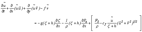 -----------------------(10)
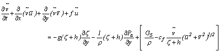 -----------------------------(11)
where ![]() =
= ![]() and
and ![]() =
= ![]() are new prognostic variables and
are new prognostic variables and ![]() gives the total depth of the basin and where over-bars denote depth averaged values, e.g.,
gives the total depth of the basin and where over-bars denote depth averaged values, e.g.,
![]()
![]()
![]()
![]()
The equation of continuity (9) along with the two momentum equations (10) and (11) form three basic equations of the numerical model. It consists of a set of three coupled equations for the unknowns ![]() ,
, ![]() , z . The forcing terms in these three equations arise out of (i) the Coriolis term, (ii) the inverted barometric changes
, z . The forcing terms in these three equations arise out of (i) the Coriolis term, (ii) the inverted barometric changes
![]()
due to fall in atmospheric pressure, (iii) the component of wind stress and (iv) the bottom stress component. However, the forcing due to barometric changes is neglected, as its effect is negligible due to small variation of pressure over the region under study.
2.3 Boundary and initial conditions
In addition to the fulfillment of the surface and bottom conditions (5) and (6), appropriate conditions have to be satisfied along with the lateral boundaries of the model area under consideration for all time. Theoretically the only boundary condition needed in the vertically integrated system is that the normal transport vanish at the coast, i.e.,
![]() for all
for all ![]() (13)
(13)
where a denotes the inclination of the outward directed normal to the ![]() - axis. It then follows that
- axis. It then follows that ![]() along the
along the ![]() -directed boundaries and
-directed boundaries and ![]() along the
along the ![]() -directed boundaries. Assuming that the motion is observed from an initial state of rest, we get,
-directed boundaries. Assuming that the motion is observed from an initial state of rest, we get,
Clearly, these equations are nonlinear in nature and an analytical solution is not possible without making major simplifying assumptions in which many important parameters may have to be dropped. The best alternative is the numerical solution. The numerical technique based on finite difference scheme consists of solving the governing equations at a discrete set of points in space at discrete instants of time. This method is also applicable when the forces and the boundary conditions are described by very complicated functions, as is almost always the case in reality. For practical forecasting, it is superior to the analytical methods.
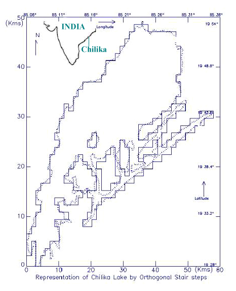
Our preliminary results are based on our numerical experiments for the analysis area shown in Fig.1 covering an extent of about 60 km and 50 km in the east-west and the north-south respectively. In order to incorporate all the islands, the coastal boundaries and the open-channels, it is required at least a minimum grid interval of about 750m. Accordingly, the Chilika lake is approximated as closely as possible to the realistic boundary of the lake. The number of grid points in the ![]() - and
- and ![]() - direction are 81 and 68 respectively and hence
- direction are 81 and 68 respectively and hence ![]() =
= ![]() =0.75 km approximately. With this grid specification, it was found that computational stability could be maintained with a time step of 60 sec. The manner of the boundary construction is illustrated in Fig. 1. The coastal boundary in the model is taken to be a vertical sidewall through which there is no flux of water. However, the lake is connected actually through two open channels. In the preliminary study, these open channels are not considered and the boundary is treated as a closed one.
=0.75 km approximately. With this grid specification, it was found that computational stability could be maintained with a time step of 60 sec. The manner of the boundary construction is illustrated in Fig. 1. The coastal boundary in the model is taken to be a vertical sidewall through which there is no flux of water. However, the lake is connected actually through two open channels. In the preliminary study, these open channels are not considered and the boundary is treated as a closed one.
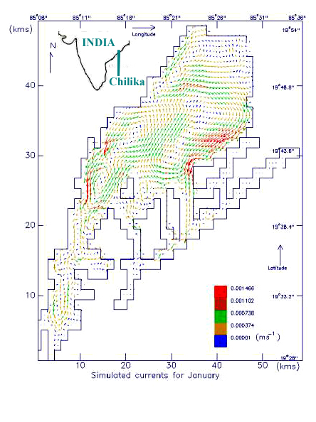
Fig. 2. Simulated currents for January
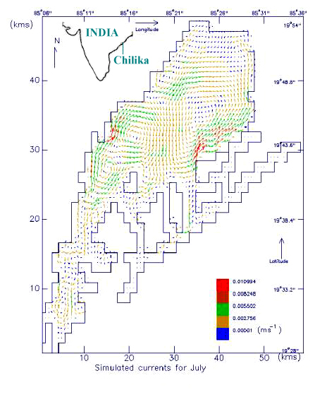
The bottom topography of the lake for January, is being generated at the model grids using spot depth observations. Accordingly, maximum and minimum water column of the lake are 2.4 m and 1.0 m respectively. In the absence of observed depths for July, we arbitrarily raised the January water level uniformly throughout the lake by 1.0 m presuming that heavy monsoon precipitation during this month would simultaneously enhance depth of the lake.
The model is forced by the climatological monthly mean winds representative of January. During this month, the direction of the wind is almost northeast with a uniform strength of 2.0 m/s over the lake. The model attains a steady state in four days. Fig 2 gives computed circulation for January with a maximum speed of about 0.2 cm/s. It is interesting to note that there are many eddies formed as a result of large variations in the bottom topography and these are responsible for the mixing process of the lake. Strong currents are noticed in the regions of strong topographic gradients. Another experiment is carried out with a mean monthly forcing of July, which is a representative for southwest monsoon. The winds for July are strong compared to January with a magnitude of about 6.5 m/s. The associated computed currents are shown in Fig. 3. It is noted that the current pattern is just reversal to that of January as a result of seasonal reversal of the winds in general in the Bay of Bengal. However, the currents are strong with a maximum magnitude of 1.4 cm/s.
The work is partly supported by the funding from Department of ocean Development, Govt.of India.
| References | up | previous | next | last |
Mohanty P. K., Panda U. S., Pal S.R. and Jayaraman G., 2002. Status of Chilka lagoon: A comparative study of pre and post mouth opening conditions (This Volume).
Nayak B. U., Ghosh L.K., Roy S. K. and Kankara R.S., 1998. A study on Hydrodynamics and Salinity in the Chilika Lake . Proceedings of the Int. Workshop on Sustainable Development of Chilika Lagoon 31 47.
Chandramohan P., Pattnaik A. K. and Jena B. K., 1998. Sediment dynamics at Chilika outer Channel. Proceedings of the Int. Workshop on Sustainable Development of Chilika Lagoon 22 30.
Hutter K., 1984. Hydrodynamics of Lakes. Springer Verlag, New York.
| Address: | up | previous |
Center for Atmospheric Sciences,
Indian Institute of Technology,
Hauz Khas, New Delhi 110 016.
Department of Marine Sciences,
Berhampur University,
Berhampur 760 007, India.