

CAUVERY RIVER: Land Use Dynamics Biodiversity & Hydrological Status
T V Ramachandra, Vinay S, Bharath S and Bharath H Aithal
IISc-EIACP, Environmental Information System, CES TE15
Indian Institute of Science, Bangalore 560012
E Mail: tvr@iisc.ac.in,
envis.ces@iisc.ac.in,
Tel: 91-080-22933099/ 23608661
Research Highlights
- Deforestation in Cauvery river catchment – Land use analysis showed that the catchment was dominated by Agriculture activities (Agriculture and horticulture) i.e., about 73.5% followed by Forest cover which is about 18%. Dense forest area was 13.3% and Degraded forest area was nearly 4.63%.
- Between 1965 and 2016, natural vegetation cover has reduced from 28194 sq.km to 15345 sq.km indicating that about 45.55% cover lost in 5 decades. dense vegetation has reduced by 35% (6123 sq.km) and degraded vegetation has reduced by 63% (6727 sq.km). Across the administrative divisions, Karnataka has lost about 57 % (9664 sq.km) followed by Tamil Nadu loosing 29% (2905 sq.km) and Kerala loosing 27% (279 sq.km) of the natural vegetation cover.
- The Pushpagiri Wildlife Sanctuary (PWLS) has not shown any changes in its vegetation cover. But, the anthropogenic pressures due to commercial crops have transformed major forests in buffer region. The shift from agriculture to horticulture and from traditional forming to rubber, tobacco, coffee cultivation has impacted on flora and fauna as well as hydrological regime of entire region.
- Talacauvery Wildlife Sanctuary (TWLS) has not witnessed any changes from 1991 to 2016 in its vegetation cover due to its high altitude forest and strict protection. Unlike core WLS the buffer region shows changes as increase in horticulture activities as a result of high rubber plantation, coffee plantations due to favorable rainfall. The existing agriculture regions were transformed for commercial plantations due to higher revenue opportunities.
- Brahmagiri Wildlife Sanctuary (BWLS) witnessed changes in the evergreen forest cover from 93.33 (1973) to 87.66% (2016). The regions near the boundary and adjacent to major roads have undergone major transitions with commercial crop activities and monoculture plantations. The shift from traditional farming to commercial crop and intensified horticulture is noticed at very high rates in buffer areas.
- Bandipur National Park (BANP) reveals a decline of 15.19 % forest cover. Eastern portions of the park have under gone major transition due to fire and anthropogenic disturbances. Native deciduous forest is converted into scrub forests (8 to 23.11 %), infested by exotic weeds, with the enhanced cattle grazing, agricultural activities.
- Nagarholé National Park (Rajiv Gandhi Tiger Reserve) reveals a decline of 11 % forest cover due to increase in human activities within the national park and in the buffer region. The buffer region is highly dominated by horticulture activities and grazing. There is a slight increase in scrub forest, rosewood, teak plantations.
- Biligiriranganatha Swamy Temple (BRT) Tiger Reserve - evergreen forest and deciduous forest cover has declined over years and there is a sharp increase in the scrub forest due to deforestation in the edges. Reduction in forest cover is also due to increase in illegal encroachment by the natives within the boundary.
- M.M. hills Wildlife Sanctuary (MMHWLS) has not witnessed any significant reduction in the evergreen forest while deciduous forest has significantly declined by 11.83% from the year 1973 to 2016 and converted into scrub forest. (14.05 %).
- Cauvery Wildlife Sanctuary (CWLS) - The vegetation cover has lost though strict protection is enforced due to population pressure and encroachments. The area under vegetation has declined by 18.43% during 1973-2016.
- Bannerghatta National Park (BNP) moist deciduous forest was covered 50.4% (1973) and now 28.5 % (2015) due to anthropogenic pressure in BNP and its environs. The BNP region has increase in agriculture area from 7.62 to 13.6 % by 2015. Forests in Ragihalli, Manjunatha, Yelavantha, Bettahalli regions with good protection measures show minimal disturbance. However, implications of unplanned urbanization are evident in the buffer regions. Land use analysis highlights of urban sprawl in peri-urban regions has fragmented, dispersed urban patches in periphery accounting to 5462 ha (built-up area). The region has 9254.21 ha of scrub forests and which can be reforested for better protection of ecosystem in BNP.
- Adichunchanagiri Peacock Sanctuary (APS) depicts major portion of the sanctuary under scrub forest cover and open areas. The scrub forest covers 61.87 % major region prone to grazing due to lack of grassy patches in the surrounding villages.
- Arabithittu Wildlife Sanctuary shows major forest cover is under scrub and grass land forest types (52.75 %), followed by deciduous cover (34.54 %) supporting herbivorous fauna effectively. The region is acting as a temporary halt for various faunal species such as Elephants migrating from Nagarholé (RTR) to other places. The agriculture shows 9% represents anthropogenic status in the region. Eucalyptus plantations in the sanctuary and its surrounding are degrading natural cover over a decade, interventions are the need of the hour to control it.
- Melkote Wildlife Sanctuary shows major cover is under scrub/ grass lands and deciduous forest. Frequent human induced forest fires in the grass lands has caused impact on regeneration of natural vegetation, which has resulted in proliferation of exotic weeds. The creation of water holes and grassy patches are to be done as priority management activity to control depredation of crops by wild animals in and around the sanctuary.
- Ranganathittu Bird Sanctuary shows 20 % area under horticulture helping the birds to nest and people are also protecting the birds without disturbing. The deciduous covers of 12.84 % dominated by trees such as tamarind, neem etc., are also helping the birds to nest. The region has some grass patches supporting as a prey base for birds.
- Ramadevara Betta Vulture Sanctuary depicts 54 % of deciduous cover followed by 12.93 % scrub forest cover. Horticulture covers 18 % of land scape and recent times old coconut plants are replaced by other commercial crops resulted in Vultures loosing habitat.
- Wayanad Wild Life Sanctuary (WWLS) - Forest constitute only 35.04 % and plantations cover 46.45 % followed by agriculture 15%. The tea estates, rubber plantations occupy major land scape region. The anthropogenic pressure is high due to many infrastructure projects and high ways.
- Mudumalai National Park (MNP) has 66.47 % of forest cover under various forest categories. Agriculture covers 23.96 % followed by plantations. The grazing and exotic weed infestations are disturbing major forest cover and ecology.
- Satyamangalam Wild Life Sanctuary (SWLS/STR) has 72.84 % under mixed forest cover ranging deciduous, thorny scrub, grass lands. The agriculture constitutes 17.75 % followed by plantations 9%. The anthropogenic pressure is because major villages are surrounded by forests and large amount of population are dependents on forest resources. The crop predation is high due to lack of resources in forests and attractive easy sugar based crops such as ragi, sugar cane etc.
- Chinnar Wild Life Sanctuary (CHWLS) has good mixed forest cover of 76.35 % due to protection. The habitat types range from shola grasslands to dry thorny scrub, across a diverse cultural landscape as well. The region is also part of Anamudi elephant reserve complex supporting rich biodiversity.
- Anamudi Shola National Park (ASNP) highlights 62.69% of evergreen (Shola) forest cover surrounded by 31 % plantations. Crop predation by wild animals is the common problem in summer due to lack of water resources in side park. The appropriate measures are need to be considered by regulatory agencies to control the exotic and commercial plantations, which are disturbing ecology.
- The flora species (486) belong to 116 families across the basin. The Lauraceae, Fabaceae, Myrtaceae, Poaceae, Rubiaceae are the dominant families found in the basin. The region has highly endemic species around (147 species) such as Artocarpus hirsutus, Atalantia wightii, Blachia umbellate, Cinnamomum macrocarpum, Cinnamomum malabaricum, Cinnamomum travancoricum, Diospyrous paniculata, Garcinia gummi-gutta, Holigarna grahamii, Hopea ponga, Ixora brachiata, Knema attenuate, Pinanga dicksonii, Syzygium densiflorum, Syzygium malabaricum, Terminalia travancorensis, Vateria indica etc.
- Serving as a prime habitat for several species of amphibians, reptiles, birds and mammals comprising Tiger (Panthera tigris), Asian Elephant (Elephas maximus), Indian gaur (Bos gaurus), Sambar deer (Cervus unicolor), Spotted deer (Axis axis), Leopard (Panthera pardus), Wild dog (Cuon alpines), Sloth bear (Melurus ursinus), Smooth coated otter (Lutrogale perspicillata), Pangolin (Manis crassicaudata), Slender loris (Loris lardigradus) and Black naped hare (Lepus nigricollis), etc.
- The elephants move from Pushpagiri Wild Life Sanctuary (PWLS) located in northern top portion of basin to Southern eastern portion of Tamil Nadu state (Satya Mangalam forest, Tali reserve forest etc.,)
- Catchment has witnessed a drastic Increase in cropping area.
- Tamil Nadu, Irrigation area has increased from 6556 sq.km (13.8%) to 20233 sq.km (42.7%) between 1928 and current decade.
- Karnataka, Irrigation area has increased from 1193 sq.km (3.42%) to 8497 sq.km (24.3%) between 1928 and current decade.
- Enhanced Water demand
- Tamil Nadu, Water demand has increased from 429 TMC to 573 TMC between 1928 and 1971.
- Karnataka, Water demand has increased from 72 TMC to 171 TMC between 1928 and 1971.
- Average annual rainfall in the Western Ghats part of Kerala varies between 2700 mm to over 3500 mm across space,
- Karnataka portion of Western Ghats receives average annual rainfall between 2500 to 5000 mm.
- Tamil Nadu inlands areas also one of the driest belt next to Karnataka portion of Deccan Plateau in Cauvery basin. This region has an average annual rainfall ranging between 640mm to 1750 mm at transition zones with coefficient of variation up to 0.22.
- East Coast of Tamil Nadu receives rain average annual rainfall between 845 mm to 1300 mm, with coefficient of variation ranging up to 0.24.
- Across the Cauvery basin, south west monsoon yields 428 TMC and North East Monsoon yields 302 TMC, Gross yield in the basin is about 786 TMC considering non monsoon showers across other months.
- Cauvery catchment in Karnataka state has an annual water yield of 348TMC of which south west monsoon caters about 68.5% of the total i.e., about 238 TMC and north east monsoon caters to 21% yield, remaining flow is due to the showers during April and May.
- Cauvery catchment in Tamil Nadu is also equivalent to that of Karnataka yielding water about 325 TMC, Tamil Nadu state receives maximum rainfall during north east monsoon i.e., about 67.7% yielding 220 TMC of water and south west monsoon contributes to 25% of the total yield i.e., about 81 TMC.
- Cauvery catchment in Kerala contributes to yield of 111 TMC of which south west monsoon contribute to 88.7% of the total yield i.e., about 98.5 TMC.
- Ground water recharge - Across the administrative divisions, Tamil Nadu has highest yield potential about 118 TMC, followed by Karnataka with 109 TMC and Kerala with 41 TMC.
- Ground Water Recharging Capability in the catchment, across the administrative divisions, Tamil Nadu has highest yield potential about 118 TMC, followed by Karnataka with 109 TMC and Kerala with 41 TMC.
- Total Domestic Demand in Cauvery basin is about 78 TMC of which Tamil Nadu state has a demand of 45 TMC, Karnataka 30 TMC, Kerala 2 TMC and Puducherry about 1 TMC. Additionally, part of domestic water demand about 180 MLD (2.3 TMC) is catered to Chennai and about 1350 MLD (17.4 TMC) is catered to Bengaluru city.
- Across the basin, livestock water demand is about 9 TMC of which Tamil Nadu has a demand of 4.8 TMC, followed by Karnataka with 3.5 TMC and Kerala with 0.1 TMC.
- Across the administrative divisions, with existing scenario of cropping, Tamil Nadu has the highest demand of 585 TMC, followed by Karnataka with 529 TMC, Kerala with 62 TMC and Puducherry with 5 TMC. Entire basins water demand with respect to agriculture is about 1180 TMC. Spatial analysis shows that Karnataka and Kerala areas under agriculture depends majorly on South west monsoon between June to September, whereas majority of Tamil Nadu is dependent on the north east monsoon
- Cauvery basin on a whole has a total demand 1267 TMC of which Tamil Nadu has a demand of 637 TMC followed by Karnataka with 563 TMC, Kerala with 64 TMC and Puducherry with 5 TMC
- Hydrological status quantified as function of supply and demand is depicted in Figure 4.6.2. Catchments in the Ghats and closer to the Ghats have better hydrological status with supply greater than 1, whereas the upstream catchment in Karnataka portion of Cauvery indicate severe stresses of water with hydrological status less than 0.5. Interior and Coastal Tamil Nadu portion of Cauvery are also under moderate stresses with existing cropping pattern.
- The basin has the capability to cater about 67% of the total water requirement with existing cropping pattern and at normal rainfall conditions.
- COV in the basin ranges between 0.12 to 0.28. Low variability (< 15%) of rainfall was observed in the Ghats and High variability (> 25%) at the plains of interior Karnataka. Coast and interior Tamil Nadu had moderate variations about 18 to 22%.
- During drought, Rainfall ranges between 364 mm and 4700 mm compared to range of 470 mm to 5500 mm across the basin, on an average, basin receives rainfall of 608 mm.
- Annual runoff in the catchment during drought year ranges between 85 mm to 830 mm across the basin. Water yield during drought in the catchment is about 535 TMC across the year of which South west monsoons contribute to 302 TMC and North East Monsoons cater to 193 TMC of yield. Across the administrative divisions, Karnataka has yield of about 245 TMC of which South west monsoon has a share of 177 TMC, Tamil Nadu has a water yield of 203 TMC of which North east monsoon contributes 141 TMC, Kerala has a yield of 84 TMC of which South West monsoons cater to 76 TMC.
- Replacing paddy with less water demanding millets and pulses during monsoon and reducing other crops by 30%. By doing this the total water demand in the basin reduced to 549 TMC against total yield about 558 TMC and all sub basins havelesser stresses compared to scenario 3.
Highlights – Problems
- Inappropriate cropping pattern - Inappropriate crops, multi season water intensive crops and inefficient use of water
- Catchment degradation without proper watershed programs. Decline in the community participation in watershed management and the absence of water and soil conservation measures
- Silted lakes and Reservoirs. Lack of de-silting of water bodies or lack of eco-management of either flood plains or buffer (afforestation measures)
- Unsustainable Sand mining in river beds
- Cauvery conundrum Erroneous assumptions, flawed estimations and irresponsible decisions – nexus of crooked politicians, greedy consultants, inefficient and incompetent bureaucracy.
- Impending climate change: Further erratic rainfall due to climate change with the global warming.
- Lack of integrated sustainable management of natural resources (land and water) in the river basin
Highlights – Solutions
- The integrated management of catchment with the interlinked natural resources like water, soils and the forest for the wellbeing as well as other forms of life -flora and fauna.
- Restrictions on large scale water intensive cash crop in the catchment and promotion of organic farming
- Arresting deforestation and enriching the catchment with native species
- Maintaining forest cover of native species
- Restrictions on monoculture either under social forestry programmes, afforestation programmes or large scale commercial plantations
- Restrictions on the over-exploitation of groundwater
- Treatment of sewage through the decentralized treatment plants (Secondary treatment plant integrated with the Constructed wetlands and algal pond as in Jakkur Lake, Bangalore)
- Setting up effluent treatment plants and ensuring zero discharge from industries
- Removal of encroachment of river bed and drains
- Mapping of flood plains and restrictions on setting up any permanent structures in the flood plains
- Maintaining the integrity of flood plains (buffer zones) and strengthening riparian vegetation of native species (which will help in enhancing the livelihood prospects while treating surface run-off)
- Environmental awareness among locals through environment education programmes at schools, colleges and at community levels
- Ban on plastics and sustainable management of solid waste at decentralized levels.
Introduction
Blue planet, the Earth [1] is abundant with natural resources supporting numerous lifeforms in terrestrial and aquatic habitats for millions of year [2]. Among all the natural resources, water is abundant covering over 70% of earth surface [3] i.e., about 1386 Million km3. Figure 1.1 depicts the land cover map of earth, indicating various land features and water bodies [4].
Water is a dynamic agent that plays multiple role in (i) evolving abiotic and biotic components on our planet (Vedic Literatures and Darwins Evolution Theory) (ii) shaping of landscapes, (iii) influences movement of energy through climate (greenhouse gas absorbing radiation and reemitting it to the surface; reflect sunlight in form of clouds, snow, and ice; transport heat energy through evaporation, circulation and condensation), (iv) distribution of earth gravity system, (v) sustaining the biotic factors (flora and fauna) [5].
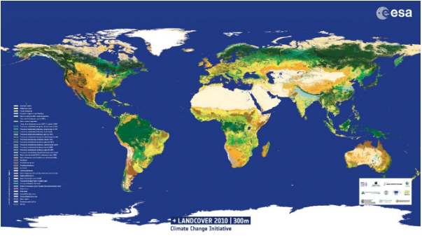
Figure 1.1: Global Land cover [4]
Among all the available natural water resource a small fraction about 2.5 – 3.0% [2], [6] of water is Fresh water resource of which 2/3rd is locked in the form of Glaciers, Snow cover [1], of the remaining 33.33% portion of fresh water, ground water contributes to 30%, remaining as streams, lakes, soil moisture, that play an important role in catering to socio-cultural, environmental needs. Figure 1.2 depicts distribution of water across globe.

Figure 1.2: World Water resource [6]
The Brisbane declaration [7] in 2007 highlights the role of fresh water and need for protecting the resource as follows
- Freshwater ecosystems are the foundation of our food, health, social, cultural, and economic well-being: Healthy freshwater ecosystems – rivers, lakes, floodplains, wetlands, and estuaries – provide clean water, food, fiber, energy and many other benefits that support economies and livelihoods around the world. They are essential to sustain water and ensurefood security, human health and well-being.
- Freshwater ecosystems are seriously impaired and continue to degrade at alarming rates: Aquatic species are declining more rapidly than terrestrial and marine species. As freshwater ecosystems degrade, human communities lose important social, cultural, and economic benefits; estuaries lose productivity; invasive plants and animals flourish; and the natural resilience of rivers, lakes, wetlands, and estuaries weaken. The severe cumulative impact is global in scope.
- Water flowing to the sea is not wasted: Fresh water that flows into the ocean nourishes estuaries, which provide abundant food supplies, buffer infrastructure against storms and tidal surges, and dilute and evacuate pollutants.
- Flow alteration imperils freshwater and estuarine ecosystems: These ecosystems have evolved with, and depend upon, naturally variable flows of high-quality fresh water. Greater attention to environmental flow needs must be exercised when attempting to manage floods; supply water to cities, farms, and industries; generate power; and facilitate navigation, recreation, and drainage.
- Environmental flow management provides the water flows needed to sustain freshwater and estuarine ecosystems in coexistence with agriculture, industry, and cities: The goal of environmental flow management is to restore and maintain the socially-valued benefits of healthy, resilient freshwater ecosystems through participatory decision-making informed by sound science. Ground-water and floodplain management are integral to environmental flow management.
- Climate change intensifies the urgency: Sound environmental flow management hedges against potentially serious and irreversible damage to freshwater ecosystems from climate change impacts by maintaining and enhancing ecosystem resiliency.
- Progress has been made, but much more attention is needed: Several governments have instituted innovative water policies that explicitly recognize environmental flow needs. Environmental flow needs are increasingly being considered in water infrastructure development and are being maintained or restored through releases of water from dams, limitations on groundwater and surface-water diversions, and management of land-use practices. Even so, the progress made to date falls far short of the global effort needed to sustain healthy freshwater ecosystems and the economies, livelihoods, and human well-being that depend upon them.
Water as a resource is extensively used across various human centric sectors such as navigation, agriculture, power generation, domestic and livestock, industries etc.[8]. Fresh water resources are depleting with increasing anthropogenic requirements have become limiting factor. Increasing abstraction of fresh water resource has led to large scale compromise and degradation in flow regime across many rivers, streams, lake, estuaries and other water systems across India and World [9]. Harnessing of fresh water resource more than the availability has led to scarcity of resource, leading to imbalance in the ecosystem, social problems (such as intra/inter-state conflicts)[10].
Twentieth Century planning and development of water resource during the twentieth century relied on various factors such as population, per capita water demand, agriculture production, socio-economic activities. These variables are ever rising, due to mismanagement and continued abuse of water bodies [11] (Figure 1.3), and has eventually lead to the over exploitation and frequent water conflicts.
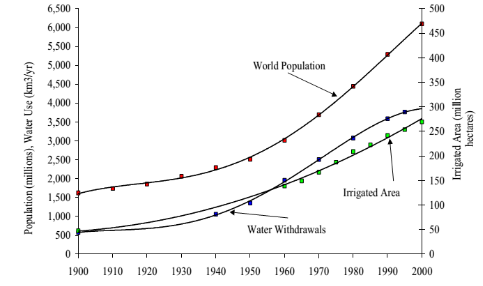
Figure 1.3: World Population, Water use and Irrigated area [11]
1.1 Water Resource in India: About 4% of the world’s fresh water resource exists in India, making India as one of the water rich nation across the globe despite which India is designated as “Water Stressed Region” [12] due to inappropriate water usage. India on an average receives nearly 120 cm annually and majorly dependent on the south west and north east monsoons [13]. Across the country there are several perennial and intermittent rivers contributing to 1953 km3 of stream flow[14], and ground water recharge potential of 342.43 km3. Table 1.1 lists the surface water yield and Table 1.2 provides ground water potential across major river basins in India [13].
Table 1.1: Surface water potential across major basin
|
Sl.no |
Name of the River Basin |
Average flow BCM/year |
|
1 |
Indus (up to Border) |
73.31 |
|
2 |
Ganga |
525.02 |
|
3 |
Brahmaputra Barak and others |
585.6 |
|
4 |
Godavari |
110.54 |
|
5 |
Krishna |
78.12 |
|
6 |
Cauvery |
21.36 |
|
7 |
Pennar |
6.32 |
|
8 |
East Flowing Rivers Between Mahanadi and Pennar |
22.52 |
|
9 |
East Flowing Rivers Between Pennar and Kanyakumari |
16.46 |
|
10 |
Mahanadi |
66.88 |
|
11 |
Brahmani and Baitarni |
28.48 |
|
12 |
Subernarekha |
12.37 |
|
13 |
Sabarmati |
3.81 |
|
14 |
Mahi |
11.02 |
|
15 |
West Flowing Rivers of Kutch, Sabarmati including Luni |
15.1 |
|
16 |
Narmada |
45.64 |
|
17 |
Tapi |
14.88 |
|
18 |
West Flowing Rivers from Tapi to Tadri |
87.41 |
|
19 |
West Flowing Rivers from Tadri to Kanyakumari |
113.53 |
|
20 |
Area of Inland drainage in Rajasthan desert |
Negligible |
|
21 |
Minor River Basins Draining into Bangladesh and Myanmar |
31 |
Table 1.2: Ground Water Potential across Basin of India
|
Sl.no |
Name of Basin |
Ground Water potential (bcm) |
|
1 |
Brahmai with Baitarni |
4.05 |
|
2 |
Brahmaputra |
26.55 |
|
3 |
Cambai Composite |
7.19 |
|
4 |
Cauvery |
12.3 |
|
5 |
Ganga |
170.99 |
|
6 |
Godavari |
40.65 |
|
7 |
Indus |
26.49 |
|
8 |
Krishna |
26.41 |
|
9 |
Kutch and Saurashtra Composite |
11.23 |
|
10 |
Tamil Nadu |
18.22 |
|
11 |
Mahanadi |
16.46 |
|
12 |
Meghna |
8.52 |
|
13 |
Narmada |
10.83 |
|
14 |
Northeast Composite |
18.84 |
|
15 |
Pennar |
4.93 |
|
16 |
Subarnrekha |
1.82 |
|
17 |
Tapi |
8.27 |
|
18 |
Western Ghat |
17.69 |
1.2 HYDROLOGICAL CYCLE:
Hydrological Cycle (Figure 1.4) describes the continuous process in which water moves above, below the earth surface and the atmosphere. It also describes the interaction of water between various earth surface features. Water cycle dynamics (Hydrological processes) plays a major role in ecological, biological, physical, and geochemical functions of a catchment [15]. Even though Hydrological Cycle is a natural process, human interventions have altered timing and functions of water resource, which in turn affected the cycle [5].
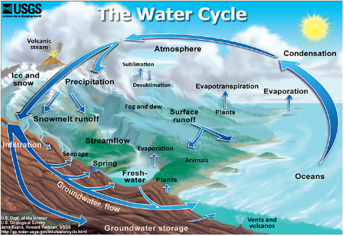
Figure 1.4: Hydrological Cycle [16]
1.3 HYDROLOGICAL PROCESSES
Precipitation: Any moisture that naturally transfer from clouds to ground could be termed as Precipitation[17]. Precipitation is an important factor in the hydrologic cycle transporting water from surface to atmosphere and vice versa. It is the input that enacts on various hydrological factors such as runoff, infiltration, ground water recharge, etc. All life forms terrestrial/ aquatic, their diversity, cropping pattern, depends on precipitation characteristics [18]–[23]. There are various factors affecting precipitation [17], [19], [24]–[28] such as
- Topography: Altitude is directly proportional to rainfall. In general, high altitude places have higher precipitation compared to low lying areas. The Ghats, followed by the coastal areas have high precipitation compared to the interiors.
- Latitude: Across latitudes, precipitation as rainfall events are very high at lower latitudes, closer to equator, whereas precipitation as snow fall is higher towards the poles.
- Temperature: Regions with higher temperature are bound to have higher precipitation since these regions have higher quantity of evaporation and transpiration aiding to from large masses of rain bearing clouds.
- Land use: Presence of natural forest cover in the region, allows large quantity of water to transpire across all months, resulting in higher precipitation. Loss of forest cover, has led to reduction in summer precipitation.
- Others: Distance from Ocean, Wind Direction.
In India, precipitation is in the form of rainfall and snow fall, about 80% of precipitation is driven by South west monsoon and north east monsoon [24]. Rivers in the north are fed by both forms of precipitation help in retaining water across all seasons, whereas in the southern part of India, rainfall presumes as sole source of water.
Runoff: During any rainfall event, a portion of water flows away as a thin sheet on the surface contributing to the streams to flow along the natural gradient known as runoff. It is also described as that portion of excess rainfall that flows away from the surface after catering to the evapotranspiration and infiltration rates[17], [29], [30]. Runoff across the globe is contributed by two major factors i.e., i) rainfall, ii) snow melt (Glaciers). Runoff is controlled [17], [29], [31] by various factors such as i) land use, ii) natural forest cover, iii) climatic factors, iv) geology, v) soil, vi) topography, vii) catchment physiology, etc. (Note: detailed explanation in the hydrological Regime Section)
Interception: Interception is a process in which part of precipitation gets collected on the vegetation surfaces and eventually gets evaporated or reaches ground as stem flow [29], [32], [33]. Interception depends on the i) vegetation characteristics such as type of vegetation, size of leaf, canopy, density ii) rainfall characteristics such as intensity, duration, size of rain drop [34]–[37]. Annually interception accounts to at least 25% of precipitation [33], [38], [39] and at least 30% of transpiration [40].
Infiltration : It is the amount of water that move laterally and vertically through the soil surfaces filling the pore spaces there by replenishing soil moisture, vadoze zone and ground water zones [17], [29]. Understanding infiltration is important since it provides the estimate of quantity of rainfall that would lead to flood like conditions. Infiltration process is dependent on [17], [41]–[43]:
- Rainfall Characteristics: Rainfall duration and intensity play a major role in defining infiltration capabilities of the land surface. Heavy down pour would lead to early surface saturation and reduce infiltration rates at shorter duration while if the rainfall rate is smaller than the infiltration capacity, saturation rates reduce with increase in infiltration duration.
- Soil Characteristics: Infiltration is affected by the surface conditions, surfaces with grass and mulch compared to bare lands have higher infiltration rates. Physical properties of soil such as texture, structure, organic content, depth of soil strata, plays a major role in defining infiltration abilities of soil. Soils such as sand have higher infiltration capability but lower water holding capacity, whereas clayey soils have lower infiltration rate but higher water holding capacities. Presence of pore spaces allows water to infiltrate at larger rates compared to dense soils.
- Vegetation characteristics: Natural forests have the ability to allow water to percolate for deep inside due to their deep root systems. These roots allow the soils to break and create more pore spaces enhancing infiltration abilities. Soil in monoculture patches are compact there by reduces infiltration rates.
- Anthropogenic Activities: Human activities altering the landscape such as deforestation, livestock grazing, agriculture disturbs the soil mass in the system and hence altering the infiltration capabilities.
Evapotranspiration: Quantity of water either as solid or liquid form that is transferred back to the atmosphere from earth surface features [44], [45] either as transpiration through vegetation or as evaporation through soil and water bodies. Evapotranspiration is one of the important process in the hydrological cycle since it is responsible for formation of water vapors which condense to from clouds, without which precipitation would fail [46]. Around 60 – 80% of precipitation is returned back from earth surface as evapotranspiration [47], [48]. The process of evapotranspiration is dependent on various factors[46] such as:
- Temperature – Temperature is directly proportional to Evapotranspiration rates.
- Humidity – Humidity is inversely proportional to evapotranspiration rates.
- Wind speed – Rate of evaporation will increase with moving winds. Moving winds will clear humidity allowing higher transpiration in plants.
- Water availability – Water availably as part of soil water plays a major role in transpiration. Dry soils with no moisture would reduce evaporation rates to zero. Plants when stressed with water would reduce transpiration rates by storing water in their stomata.
- Soil type – Soil texture determines the water holding capacity. Clayey soil has high water holding capacity whereas sandy soils low water holding capacity. Density/Compactness of soil also plays a major role in determining available water to plants to transpire.
Vegetation type – Deciduous plant species shed their leaves to conserve water against transpiration, whereas evergreen species allows transpiration throughout the year. Cactus Species do not transpire much compared to other plant species.
1.4 FACTORS AFFECTING HYDROLOGICAL REGIME
LAND USE is refereed as the various ways in which mankind uses and manages the land surface resource such as development, conservation, irrigation, mixed use etc. [1] or based on natural phenomenon’s forests, rivers, oceans, open lands, glaciers etc. [2]. The heterogeneous pattern (structure and composition) of land use elements, land forms, vegetation type etc. interacting each other defines a landscape [51]–[56]. Landscape and its development is an outcome of natural processes such as interaction of climate, colonization of flora and fauna, formation and development of soils (minerals) across strata and disturbances [57], [58]. Cluster of landscape forms small watersheds and combination of these smaller watersheds forms larger watersheds or basins [59]. Landscape heterogeneity is linked with ecological and economical values [60] such as interaction of spatial elements, cycling of water and nutrients, bio-geo-chemical cycles, climatic factors, etc. This highlights that the functional aspect of ecosystem depends on the structure (shape, size, configuration) and pattern (linear, regular, aggregated, space) of the landscape. Alterations in the land use at global or local level either through natural or cultural (anthropogenic) forces can alter the functioning capability of landscape resulting in ecological, economic and environmental consequences threatening sustainability and multi-function-ability of the natural resources [61]–[64]. In this context, landscape changes are seen as threat or negative evolution since the current changes are directly proportional to the loss of habitats, corridors, bio-diversity, coherence, climate change and depletion of natural resources [65]. Understanding of landscape can be brought under three principles of landscape ecology [59]viz.,
- Time and Space: Landscape elements are both spatially heterogeneous and temporally heterogeneous (process and changes across time scale) [66] . Effect on/of landscape and/on ecology can always be studied across seasons, years or decades as well as across a small area such as small watershed to large river basins supporting large range of ecosystems[67]. Generally, effect of any disturbances can be studied based on the principle of time and space, which would help in conceptualizing sustainable development framework.
- Heterogeneity: Defines the diversity within the landscape. For any ecosystem to survive and function, it necessary to have heterogeneous landscape [56], the diversity allows the ecosystems to survive stresses across climatic conditions.
- Connectivity: Connectivity within or between landscapes serves as movement path (corridor) that helps in transfer of nutrients, energy between flora and fauna [68]. Conditions corridor of natural vegetation provides essential connection between management sectors distributed across large landscapes [69].
These principles of landscapes, and their dynamics across space or time, patterns, connectivity etc. with their functions can be understood by means of spatiotemporal pattern analysis [54] involving remote sensing and Geographical Information System [70]–[73].
Remote sensing technology is used as source of data for characterizing land use and land cover information at local to global scales [74]. Remote Sensing is a process of acquiring, processing and interpreting data to derive information about an object, landscape or process/phenomenon from a distance [71], [75]. The process of obtaining information about an object or the landscape is by measuring the amount of emitted or reflected electromagnetic energy from the object/surface using sensors mounted on air or satellite based platforms and through image processing techniques [70], [76].
Remote Sensing is defined in various ways
- Science of Acquiring, Processing and Interpreting images and related data obtained from aircraft [70]
- Science and Art of obtaining information about an object, area or phenomenon through analysis of data acquired by the device that is not in contact with the object, area or phenomenon under investigation [71].
- Acquisition of information about an object without being in physical contact with it [77].
- Art and Science of making measurements of the earth using sensors [78].
- Science, Art and Technology of obtaining reliable information about physical objects and the environment, through the process of recording, measuring and interpreting imagery and digital representation of energy patterns derived from non-contact sensor system [79]
Based on various definitions Remote sensing can be considered as the Art, Science, Technology, for Acquiring, Processing and Interpreting data to derive information about the object. The process of remote sensing can be broadly split into two broad categories [71] i.e.,
- Data Acquisition: The process of data acquisition involves various elements such as
- Propagation of energy through the atmosphere (Incoming Solar radiations or electromagnetic waves)
- Energy interaction with earth surface features (absorption, emission, diffusion, reflection of the radiations)
- Retransmission of energy through the atmosphere
- Airborne or Space borne sensors to receive the emitted electromagnetic radiations and store the data.
- Re-transmission of data from sensors to ground stations where the data is stored as analog (image) or digital (digital number) form.
- Data Analysis:
- Examining the data received from space borne sensors and applying suitable rectifications (radiometric/geometric).
- Geographically referencing data.
- Extracting information based on reference datasets based on visual interpretation or digital image processing techniques based on spectral signatures.
- The information is stored as Maps/Tables/Layers that are further used with other layers in a Geographical Information System for decision making, monitoring, etc.
Geographical Information System (GIS) can be defined as a set of tools for collecting, storing, retrieving, transforming, relating and displaying spatial data in association with database for particular set of purposes [71], [73]. GIS based data represents the real word in terms of (i) position, through (ii) attributes and (iii) relationships. GIS is a multidisciplinary since it has the ability to involve Database Management Systems, Mathematical operations, Modeling abilities, involving Bio-Geo-Chemical aspects.
Considering the abilities of geo-informatics (Remote Sensing and GIS), and integrating [80]–[82] them have been successfully used in various sectors such as i) disaster management, ii) planning, iii) forest, iv) geology, v) geography, vi) agriculture, vii) transport, viii) habitat mapping, ix) modeling/prediction, x) water resource management, xi) waste management, xii) pollution, etc [62], [64], [83]–[89].
Forest Vegetation: Forests play a major role in maintaining the hydrological regime with multitude effects in catchment [90]. Forests captures water from the atmosphere increasing rainfall and condensing fog. The process of capturing water alters with canopy height, canopy roughness, forest maturity, diversity, disturbance [91]. Forests regulate/stabilize water flow in the streams/rivers [92], forest floors act as sponge retaining water hence reducing the quantity if peak flows [93], and increasing sub surface base flows. Large forest expanses and maturity reduces peak flows and surface runoff yields [64], [94]–[97]. Water storage in the sub surfaces and controlled release is due to the tree roots grow into cracks and aid in the breakdown of bedrock, penetrating compact soil layers, allowing soil aeration and water infiltration. Vegetation cover over an area creates a micro climate modifying temperatures, moisture conditions under the canopy [98].
Anthropogenic activities (Land use changes): In the process of catering anthropogenic requirements, large scale landscape changes occur over time, involving water abstraction/retention to cater domestic, industrial, agriculture, power generation requirements. Major changes in land use that affect hydrology are afforestation and deforestation, intensification of agriculture, draining of wetlands, road construction, and urbanization [99].These anthropogenic activities have direct impact on the hydrological regime (such as rainfall pattern, runoff, evapotranspiration, reducing ground water recharge, infiltration, soil water conductivity/pore spaces ) [100]–[102] . Abstraction of water through construction of diversion channels, dams, etc. effect the hydrological regime as described in Table 1.3.
Table 1.3: Human impacts on hydrological regime and ecosystem [103], [104]
|
Sl.no |
Activity |
Impacts |
|
1 |
Dam construction, Flow diversion |
Alters timing, blocks river passage, quantity of river flow, reduces replenishment of nutrients, sediments, block fish migration, reduced aquatic diversity |
|
2 |
Draining of wetlands |
Eliminates the key components of the aquatic ecosystem |
|
3 |
Deforestation / land use change |
Alters runoff pattern, recharge capabilities lost, higher sedimentation. |
|
4 |
Release of waste water |
Diminishes water quality and associated aquatic habitats |
|
5 |
Introduction of exotic species |
Eliminates native species, alters production and nutrient cycle. |
Catchment land use influences hydrographs (peaks and falls), explaining variation in bio-physical sensitive to flow regime [105]. Figure 1.5 depicts the role of landscape on the hydrological regime. Catchments with higher proportion of natural forest /vegetation would have lower erosion and sedimentation rates, higher recharging capability higher ground water yield, whereas catchments with disturbed landscape have lower infiltration capabilities, higher surface runoff which allow pollutants, sediments to be carried downstream chocking drainages, increase in the overland flow (quick flow) would result in floods washing away stream banks, river bed, etc. affecting the habitat [106].

Figure 1.5: Land use and Hydrograph [106]
GEOLOGY: In any catchment, similar to vegetation, geology plays a major role in defining the hydrological regime. Soil/rocks/substrata play an equal role in controlling stream flow across time. Soil acts as sponge to take up and retain water [107]. Soils allow water to flow laterally and vertically filling up the pore spaces, vertical flows recharge the ground water table, whereas the lateral allow stream to flow when rainfall recedes. Depth of soil and texture of soil controls the water holding capacity. Sandy soils have higher infiltration capability but less water holding capacity, whereas clay soils have higher water holding capacity and lower infiltration capacities [108]. Presence of organics in soil creates more void spaces allowing water to seep and store in the sub stratum. Similarly rocks below the soil layer are permeable [109] allowing portion of water to reach deep aquifers. Pervious and porous rocks allow larger quantity of water to pass through as against dense rocks[110]. Figure 1.6 depicts the hydrograph with respect to permeability capability soils and rocks in the catchment. Impermeable rocks/soil lead to sharp peak in overland flow as against permeable surface.

Figure 1.6: Hydrograph of permeable and impermeable rock/soils [111]
1.8 TOPOGRAPHY (MORPHOLOGY): Topography is one among the five elements (Meteorology, Soil, Land use, Topography, Stream Network) influencing the hydrological regime [112]. Generally, topography is a permanent characteristic and influences the concertation time in basin [113]. Topography defines channel morphology (such as shape, size, slope, drainage pattern, channel width depth etc.,) land use, vegetation of catchment.
Size: Size of a catchment is an important factor in runoff yield/ hydrograph. Volume of discharge is proportional to the size of catchment [114], [115]. Larger basins will have larger reach time/lag time compared to small streams. Peak flow per unit area will decrease with increasing catchment size [116]. Figure 1.7 depicts the stream flow characteristics with respect to catchment size.

Figure 1.7: Catchment size and Hydrological regime [111]
Shape: Shape of any catchment have a definite impact on the hydrological regime. Shape, similar to size defines the lag time in any hydrograph. Fern shaped/elongated catchments require longer concentration time considered to a circular catchment. Irregular catchments can lead to multiple peaks with same rainfall event as against regular catchments. Though the runoff quantity could be the same, the hydrographs would have different peak [115]. Figure 1.8 depicts the relationship between catchment shape and hydrographs. A pear shapes catchment will have the hydrograph skewed to left with fast rising limb and high concentration at peak, fan shaped hydrograph skewed to right indicating a slow rising limb, irregular catchment with multiple peaks in hydrographs., elongated catchment with have stable flow for longer duration, whereas circular catchments hydrographs are bell shape with highest peak flow.
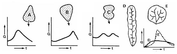
Figure 1.8: Catchment shape and Hydrological regime [117]
Slope: Catchments with large slopes generate higher velocities compared to catchments with smaller slopes, discharging larger quantity of water in shorter time [115]. Catchments with gentle slopes, balance the quantum of rainfall and runoff, storing water temporally over large areas and draining out over time. Generally, when slopes are high and variable, stream networks are dense, whereas along gentle slopes, interconnected water storage structures such as ponds, lakes, etc. are abundant. Vegetation also follows topographic pattern, i.e., in general hill tops and high slopes are contained with Grasslands and shola forests followed by evergreen/deciduous/ scrub jungles.
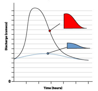
Figure 1.9: Catchment slope and Hydrological regime [118]
Drainage: Drainage pattern has an important role in defining the hydrographs. Drainage density has a direct impact on lag time and hydrograph peak [119]. For a rainfall event, basins with high drainage densities will have relatively rapid response time (shorter lag time) and steeper limbs as against low density drainages, i.e., precipitation gets into streams quicker in high dense drainages, in contrary for catchments with low dense drainages, precipitation has to travel as surface runoff, base flow, pipe flow, through fall enhancing lag time [114], [120], [121]. Various factors affecting drainage density are:
- Geology and Soil: Impermeable surfaces have high drainage densities
- Land use: natural vegetation increases interception and reduces drainage density
- Tributaries: with increasing order of stream, gradual reduction in density
- Precipitation: higher the precipitation, higher the drainage densities
- Relief: higher with steeper slopes
Description of some of the drainage patterns [122]–[126] are as below:
- Dendritic: These drainage patterns are most common across the
globe, and are associated with areas of homogeneous lithology, horizontal or very
gently dipping strata, flat and rolling extensive topographic surface having
extremely low reliefs. When a region is homogenous offering no variation in the
resistance to the flow of water, the resulting streams run in all directions without
definite preference to any one particular region. Dendritic Patten evolve with
lithological evolution i.e., erosion, sedimentation. (Figure 1.10). The tributaries
in Dendritic Patten join at low angles to the main stream or to the higher order
stream.
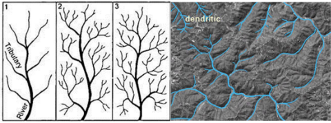
Figure 1.10: Dendritic Pattern of Drainage [123], [126] - Trellis: The trellis drainage pattern develops when the i)
underlying rock is strongly folded or sharply dipping, ii) subparallel streams erode
a valley along the strike. Longer streams will have preference to one particular
orientation, the tributaries often join the main stream at right angles which are
controlled by joints/faults. The trellis system, streams generally follow the trend
of the long, parallel valleys (Figure 1.11), short tributary enter the main channel
at sharp angles. Trellis are concentrated in areas with structural lineaments are
predominant
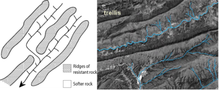
Figure 1.11: Trellis Patten of Drainage [126], [127] - Radial: Develops around a central elevated point. The drainage
pattern from dome structures, volcanic cones, batholiths and laccoliths, residual
hills, small tablelands, mesas and buttes, and isolated uplands is of radial type
where the streams emanate from a central focus and flow radially outward (Figure
1.12). These drainage systems resemble spokes of a wheel.
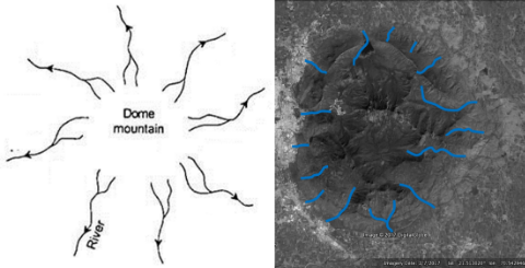
Figure 1.12: Radial Drainage [123], [128] - Parallel and Sub parallel: The internal geological structure of the
land, sometimes the parallel and sub parallel patterns are formed. The most of the
streams run in the same direction is the main characteristic feature. Tributary
streams tend to stretch out in a parallel-like fashion following the slope of the
surface, these kinds of drainage patters are found in regions of parallel, elongate
landforms like outcropping resistant rock bands, deltas, coastal plains (Figure
1.13).
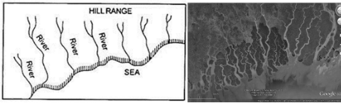
Figure 1.13: Parallel and Sub Parallel Drainage pattern[123], [128] - Annular: The streams, which form in the weaker strata of the dome
mountain, indicate approximately circular or annular pattern resembling in plan
a ring like pattern (Figure 1.14). Developed over a mature and dissected dome
mountain characterized by a series of alternate bands of hard and soft rock
beds. The annular pattern may be treated as a special form of trellis
pattern.
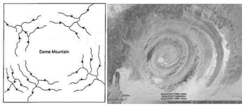
Figure 1.14: Annular Drainage pattern [123], [128] - Rectangular: A region consisting of many rectangular joints and
faults may produce a rectangular drainage pattern with streams meeting at the right
angle. Rectangular pattern is similar to Trellis, but the tributaries are widely
placed. Drainage patterns are marked with right angle bends and junctions
(Figure 1.15)
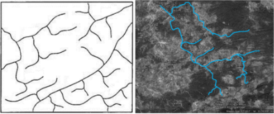
Figure 1.15: Rectangular Drainage Pattern[123], [128] - Pinnate: In pinnate stream pattern, all the main streams run in one
direction with the tributaries joining them at acute angles. These patterns are
usually found along the narrow valleys, resembling veins of leaf (Figure
1.16). These are similar to dendritic drainage pattern but are elongated in
shape.
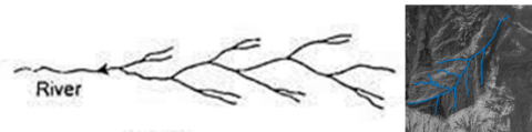
Figure 1.16: Rectangular Drainage Pattern[123], [128]
1.10 CLIMATIC VARIABLES: Climatic factors that define the flow regime are Rainfall intensity and duration, Spatial Rainfall distribution, Direction of Storm, Type of Precipitation
Rainfall/Precipitation Intensity and Duration: Rainfall intensity and duration has a direct relationship with flow regime (flow rates, flow duration, peak flows) [17]. Higher rainfall intensities will increase the peak discharge and runoff volumes in the stream/river, i.e., rainfall intensity higher than the soils infiltration capability. Similarly, if rainfall intensity is constant over certain duration, then the duration of rainfall defines peak flow and runoff volumes. If the storm duration is long enough, most of the precipitation goes away as runoff and peak flow will approach maximum rate (product of rainfall intensity and catchment area).
Rainfall Spatial Distribution: Higher rainfall near the mouth of catchment would lead to rapid rise and fall of hydrograph (Sharp peak), if the rainfall occurs at the upstream of the catchment, hydrographs would have a gradual rise with broad peak in hydrograph[17], [29], [116].
Direction of Storm: Direction of Storm has a direct effect on the catchment run off (Hydrograph). Movement of storm along the flow direction would result in high peak and shorter flow duration, whereas direction of storm as against the flow direction would result in low peak and longer flow duration [129], Figure 1.17 depicts hydrographs in relation with direction of storm.
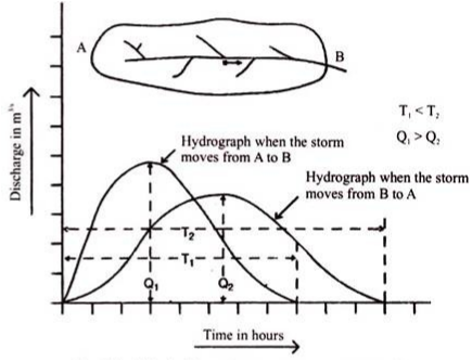
Figure 1.17: Direction of Storm and Hydrographs[129]
Type of Precipitation: Precipitation in the form of Snow would not lead to instantaneous runoff, whereas Cyclone/Thunderstorms would lead to high flows (peak and volume). Snow meld would produce runoff of similar intensity for a longer duration (broad hydrographs) as against precipitation (sharp hydrographs). Precipitation in form of mist/drizzle allows larger sub surface storage and ground water recharge.
Temperature: Temperature increase can cause either increase or decrease the volume of flow in a catchment i.e., in a Snow/Glacier fed river discharge increases with increase in temperature [130], [131] whereas decrease in flows in rain fed rivers with intense evaporation and transpiration.
1.11 ECOSYSTEM AND BIODIVERSITY INTERACTIONS
Ecosystems are distinct biological entities, determine the biogeochemical processes that regulate the Earth system, biological diversity present, productivity. Biodiversity describe varied biological organisms present at a variety of different scales, play essential roles in ecosystems. The earth’s biota is its inexplicable diversity, assessed to include about 10 million different species. The understanding of relationship between biodiversity and ecosystem functioning has emerged as a central issue during the past two decades. An ecosystem function is highly sensitive to variations in biodiversity that depicts a direct linear relationship between species richness and some measure of ecosystem functioning like productivity, biomass, nutrient cycling, carbon flux or nitrogen use [132], [133]. Biodiversity plays a crucial role in maintaining stable and productive ecosystems as natural ecosystems are defined by many interconnected processes and responsible for multi-functionality (ecosystem goods and services) [134]. Many other factors influence the magnitude and stability of ecosystem, including climate, geography, and soil or sediment type. These abiotic factors controls, interact with functional traits of species that influence in both terrestrial and aquatic ecosystem functionalities [135]. The species diversity and their interaction adds another dimension in understanding health and function of ecosystem as positive interactions among species of varied genepool influence on ecosystem responses [136]. Global biodiversity is changing at an unprecedented rate impacting strongly linked to ecosystem processes and use of natural resources. The potential ecological consequences of biodiversity loss have aroused considerable interest due to increase in domination of anthropogenic activities, species additions through biological invasions, that steadily transforming them into degraded systems [137]. These high magnitude changes have altered ecosystem functioning and stability and likely to be significantly altered diversity. The loss through natural or anthropogenic disturbances at local and global scales could threaten the stability of the ecosystem services on which humans depend [138].
The conservation and sustainable management of ecosystems are the vital components in the pursuit of development goals that are ecologically, economically and socially sustainable. The conservation and management of ecosystem has originated subsequently through realization of anthropogenic influence on ecosystem, biodiversity loss across the globe. The goals of conservation and management require strategies for managing whole landscapes including areas allocated to both production and protection. This requires an understanding of the complex functioning of ecosystems, and recognition of the full range and diversity of resources, values and ecological services that they represent, with the ability to significantly influence climate at local as well as at the global scale [139], [140]. A more systematic approach is required to identify and designing management strategies for conservation for the protection of biodiversity, including ecosystems, biological assemblages, species by realizing future demand on natural resources and numbers of people depend on them. Species composition, richness, evenness, and interactions influence ecosystem process. The detailed knowledge is the need of the hour for integration, understanding how communities are structured, controls ecosystem processes. The ecosystem management requires further understanding of the social and economic constraints of potential practices needs to be integrated with our ecological knowledge.
Conservation has become challenging task with the increase in population and development thrust. The planning for conservation pose broad challenges such as strong understanding of process, pattern and dynamic threats (natural or anthropogenic) [141]. Systematic conservation planning approach has become prime way of protecting biodiversity by have been efficient allocation of the scarce resources over past three decades. This approach includes identifying, configuring, implementing and maintaining prime areas of conservation based on resource availability and their response to the situation of vulnerability. Conservation planning is inherently spatial managed to promote the persistence of biodiversity and other natural values [142]. Conservation planning approach should cover specific elements such as identifying, mapping, and protecting rare endemic species (and particularly “hotspots” where occurrences are concentrated), watersheds with high biological values, imperiled natural communities, and other sites of high biodiversity values [143]. It should also focus consideration of habitats their natural values and conservation of focal species which includes identifying and protecting key habitats of wide ranging species and others of high ecological importance or sensitivity to disturbance by humans. Scientific understanding and sustainable resource allocation is prime consideration for effective conservation planning. Conservation should also need to focus on communicating more effectively with practitioners and stakeholders and engaging them in long-term collaborations to promote effective implementation.
The protected areas (PA), national parks (NP), sanctuaries, nature reserves, wildlife refuges, wilderness areas are created as a strong measure of conservation for protecting native habitat, biodiversity and endemic species across the globe. PAs are the foundation of conservation efforts formed as a strategy to protect and maintenance of biological diversity, natural and associated cultural resources which are managed through legal or other effective means from extinction especially those on the brink of extinction [144], [145]. Globally, establishing PAs has gained impetus for conservation and according to the International Union for the Conservation of Nature [146], nearly 13% of the global land surface is now under some form of protection. International union for conservation of nature[146] defines PAs as those areas recognized, dedicated and managed via legal policies, thus, achieving long term conservation of ecosystem and cultural values. PAs are also considered as Eco-Sensitive Areas, which can be defined as bio-climatic unit in which changes are irreversible in biological communities and their natural habitat [147]. PAs and surroundings (buffer regions) are required as they are home to many rare, vulnerable and critically endangered species thus, conserving the diversity. PAs constitutes wildlife sanctuaries, national parks, conservation and community reserves. National Park are areas of land set aside for native plants and animals. Wildlife Sanctuary is an area of ecological, floral, faunal and natural significance. Wildlife Sanctuary is declared for the protection of wildlife species present in the region [148]. Conservation Reserves and Community Reserves are the areas which acts as buffer zones, migratory corridors or connectors between the notified national park and wildlife sanctuaries. Agricultural encroachment, poaching, and illegal trade of resources are ongoing to take a toll on species, disturbing habitats, where the trees remain but the wildlife has gone. Many threatened species are continuing to survive only in protected areas, such as the Asian rhino populations preserved in Kaziranga National Park, India. PAs network is a way of maintaining natural ecosystems in the face of development pressures, rapid agricultural expansion, and a rush to exploit mineral resources. Maintaining natural forest cover is the most effective way of securing water supply, quality and reduction of floods. Protecting natural wetlands can also provide absorption space for floodwaters and help regulate water flow [149]. Healthy forest cover within PAs will enhance flora, fauna diversity and density by sustaining viable populations with reduced risks of local extinction, or by providing more complex vegetation structure for a wider range of ecological niches to support more species [150]. Land use land cover (LULC) mapping and monitoring of PAs can serve as important indicators of assessing landscape health and environmental status, distributions, and patterns [151].
1.12 ENVIRONMENTAL FLOW AND ITS IMPORTANCE
Fresh water resources since historic times have shaped the physio-biological features on earth with constant interaction with biotic (flora and fauna) and abiotic (terrain, minerals, chemicals, rock types etc.) resulting in the eco system functioning such as energy transfer between aquatic and terrestrial habitat and vice versa [103]. Flow is a master variable in any river / stream catchment since it has direct impact on the aquatic biodiversity, river morphology, river connectivity, biotic life and water quality [130], [152], [153]. Rivers, Streams and Wetlands need certain amount of water to support the aquatic health, ecosystem and biodiversity. The fresh water flows in terms of quantity and timing are essential to maintain the process and functioning of fresh water resource[154], [155]. The ecological integrity of river ecosystems depends on their natural dynamic character [156]. Over exploitation of these fresh water resources to cater irrigation, power, agriculture, industrial and other societal needs have led to degradation of perennial resource turn intermittent/seasonal in India and across the globe [9] altering the flow regimes hampering the physical, biological, hydrological functions and sustainability of resource. Based in the idea that the health of the river (water bodies) deteriorates if the flow is below a threshold the concept of minimum flow in rivers came into practice in 1970s, since then various studies have been carried out to understand the various elements of the natural flow. The concept of environmental flow was developed to understand, check the negative impact of large scale withdrawals of water from a natural system. These natural flows/ minimum flows are referred to as Environmental Flows that are necessary to maintain the health and biodiversity of water bodies, including rivers, coastal waters, wetlands and estuaries.
Environmental flows have been defined in various ways
- Quantity, timing, and quality of water flows required to sustain freshwater and estuarine ecosystems and the human livelihoods and well-being that depend on these ecosystems [7]
- Water regime provided within a river, wetland or coastal zone to maintain ecosystems and their benefits where there are competing water uses and where flows are regulated [157]
- Quantity, timing, duration, frequency, and quality of flows required to sustain freshwater, estuarine, and near shore ecosystems and the human livelihoods and wellbeing that depend on them [158]
- Minimum flow has to be maintained within a river, wetland, or coastal zone to maintain ecosystems and the benefits they provide to people and the environment [159], [160]
In general, Environmental flow can be understood as “Managing altered water resources by mimicking the natural flow regime to cater societal benefits without compromising on environmental needs”.
Analysis of Environmental flow in streams and rivers are necessary to ensure that the need of humans and that of environment are met, based on which other potential users such as industries etc., can be accommodated to abstract water [161], in determining the health of river [162], manage flow and protect the water bodies and river networks[160], maintain and enhance the ecological character and functions of floodplain, wetland and riverine ecosystems that may be subject to stress from drought, climate change or water resource development [157], [163]. Fresh water flowing into the sea has for a long time been considered a wastage of a precious natural resource understanding Environmental flow helps to understand various functions of the river (Table 1.4).
Table 1.4: Function of River [159], [164]
|
Sl.no |
Function |
Description |
|
1 |
Carrier functions |
|
|
2 |
Production functions |
|
|
3 |
Regulation functions |
|
|
4 |
Information functions |
|
Objective
Over exploitation, improper allocation and mismanagement of watershed has led to alteration of the hydrological regime of surface and subsurface water resource, would affect the water retention capability of the catchment, biota and their habitat.
The objective of the study is to
- Understand land use dynamics and Hydro-dynamics in the catchment.
- Assess Demand in Various Sectors.
- Computation of Hydrological Status
Materials and Method
3.1. STUDY AREA
River Cauvery (ಕಾವೇರಿ-Kaveri) lifeline of South India, it is also known as Dakshina Ganga[1]. River Cauvery is the east flowing river originating at Talakaveri (Kodagu-Karnataka) in the Western Ghats, flows for a distance over 770 km [2]–[4] joining Bay of Bengal near Pazhaiyar (Nagapattinam-Tamilnadu) [5] (Figure 3.1.1).. Cauvery river has a catchment area over 85300 sq.km extending across the States of Karnataka, Kerala, Tamil Nadu and Union Territory of Pondicherry (Figure 3.1.2). The basin as per the Central Ground Water Board [6] is classified as Upper Cauvery Sub basins, Middle Cauvery Sub Basin and Lower Cauvery sub basins (Figure 3.1.2, Table 3.1.1).

Figure 3.1.1: Cauvery Basin, Origin at Talakaveri and Meets Bay of Bengal at Pazhaiyar
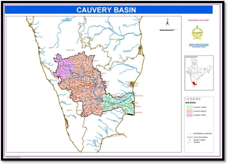
Figure 3.1.2: Cauvery basin - Sub basins and Administrative boundaries [6]
Table 3.1.1: Cauvery Sub basins [6]
|
Sub-basin |
Watershed code |
Name of Stream |
Toposheet no |
Sharing state |
Area (sqkm) |
|
Cauvery lower |
CVRL001 |
Cauvery |
58i,j |
Tamil Nadu |
2237 |
|
Cauvery lower |
CVRL002 |
Koratiyar |
58j |
Tamil Nadu |
1526 |
|
Cauvery lower |
CVRL003 |
Cauvery |
58i,j |
Tamil Nadu |
1995 |
|
Cauvery lower |
CVRL004 |
Cauvery |
58i,j |
Tamil Nadu |
1823 |
|
Cauvery lower |
CVRL005 |
Marudayar |
58i,j,m,n |
Tamil Nadu |
2196 |
|
Cauvery lower |
CVRL006 |
Kolli dam, Arasalar |
58m,n |
Tamil Nadu |
1919 |
|
Cauvery lower |
CVRL007 |
Tirumalai Ranjan, Maniyar |
58m,n |
Tamil Nadu |
1761 |
|
Cauvery lower |
CVRL008 |
Venar, Vettar |
58n |
Tamil Nadu |
1039 |
|
Cauvery lower |
CVRL009 |
Konnanar |
58m |
Tamil Nadu |
2155 |
|
Cauvery lower |
CVRL010 |
Adappa |
58n |
Tamil Nadu |
750 |
|
Cauvery middle |
CVRM001 |
Shimsha |
57c |
Karnataka |
569 |
|
Cauvery middle |
CVRM002 |
Shimsha |
57c |
Karnataka |
783 |
|
Cauvery middle |
CVRM003 |
Shimsha |
57c,d |
Karnataka |
1036 |
|
Cauvery middle |
CVRM004 |
Shimsha |
57c,g |
Karnataka |
924 |
|
Cauvery middle |
CVRM005 |
Shimsha |
57c,g |
Karnataka |
785 |
|
Cauvery middle |
CVRM006 |
Arkavati, Kundvathi |
57g |
Karnataka |
743 |
|
Cauvery middle |
CVRM007 |
Arkavati, Kundvati |
57g,h |
Karnataka |
877 |
|
Cauvery middle |
CVRM008 |
Shimsha |
57c,d,g,h |
Karnataka |
753 |
|
Cauvery middle |
CVRM009 |
Shimsha |
57d,h |
Karnataka |
744 |
|
Cauvery middle |
CVRM010 |
Shimsha |
57d,h |
Karnataka |
584 |
|
Cauvery middle |
CVRM011 |
Cauvery |
57d |
Karnataka |
884 |
|
Cauvery middle |
CVRM012 |
Shimsha |
57d,h |
Karnataka |
992 |
|
Cauvery middle |
CVRM013 |
Cauveri |
57d |
Karnataka |
411 |
|
Cauvery middle |
CVRM014 |
Kabini |
57d |
Karnataka |
336 |
|
Cauvery middle |
CVRM015 |
Kabini |
57d, 58a |
Karnataka |
718 |
|
Cauvery middle |
CVRM016 |
Kabini |
57d, 58a |
Karnataka |
563 |
|
Cauvery middle |
CVRM017 |
Kabini |
49m, 58a |
Karnataka, Kerala |
945 |
|
Cauvery middle |
CVRM018 |
Kabini |
49m, 58a |
Kerala |
1226 |
|
Cauvery middle |
CVRM019 |
Akravati, Swarnamuikhi |
57g,h |
Karnataka |
856 |
|
Cauvery middle |
CVRM020 |
Akravati |
57h |
Karnataka, Tamil Nadu |
979 |
|
Cauvery middle |
CVRM021 |
Shimsha |
57h |
Karnataka |
798 |
|
Cauvery middle |
CVRM022 |
Shimsha |
57d,h, 58e |
Karnataka |
674 |
|
Cauvery middle |
CVRM023 |
Cauvery |
57d,h, 58e |
Karnataka |
1070 |
|
Cauvery middle |
CVRM024 |
Kabini |
57d |
Karnataka |
430 |
|
Cauvery middle |
CVRM025 |
Kabini |
57d, 58a |
Karnataka |
555 |
|
Cauvery middle |
CVRM026 |
Kabini, Nugu hole |
57o, 58a |
Karnataka, Tamil Nadu, Kerala |
1288 |
|
Cauvery middle |
CVRM027 |
Kabini, Gurdal |
57d, 58a |
Karnataka |
1021 |
|
Cauvery middle |
CVRM028 |
Swarnavati |
57a, 58e |
Karnataka, Tamil Nadu |
1347 |
|
Cauvery middle |
CVRM029 |
Swarnavati |
57d,h, 58a,e |
Karnataka |
519 |
|
Cauvery middle |
CVRM030 |
Chinnar |
57h,l |
Tamil Nadu |
824 |
|
Cauvery middle |
CVRM031 |
Arkavati |
57h |
Karnataka, Tamil Nadu |
736 |
|
Cauvery middle |
CVRM032 |
Cauvery |
57h |
Karnataka |
493 |
|
Cauvery middle |
CVRM033 |
Vauvery |
57h |
Karnataka, Tamil Nadu |
1373 |
|
Cauvery middle |
CVRM034 |
Udutral Halla |
57h, 58e |
Karnataka, Tamil Nadu |
812 |
|
Cauvery middle |
CVRM035 |
Palai Maleru |
57h, 58e |
Karnataka, Tamil Nadu |
967 |
|
Cauvery middle |
CVRM036 |
Palai Maleru |
57h, 58e |
Karnataka, Tamil Nadu |
771 |
|
Cauvery middle |
CVRM037 |
Bhavani |
58e |
Tamil Nadu |
1511 |
|
Cauvery middle |
CVRM038 |
Moyar |
58a,e |
Tamil Nadu |
561 |
|
Cauvery middle |
CVRM039 |
Moyar |
58a |
Karnataka, Tamil Nadu |
1072 |
|
Cauvery middle |
CVRM040 |
Bhavani |
58a,e |
Tamil Nadu |
1298 |
|
Cauvery middle |
CVRM041 |
Kunda |
58a |
Kerala, Tamil Nadu |
1203 |
|
Cauvery middle |
CVRM042 |
Chinnar |
57h,l |
Tamil Nadu |
759 |
|
Cauvery middle |
CVRM043 |
Nagavati, Vellar |
58e,i, 57h,l |
Tamil Nadu |
1019 |
|
Cauvery middle |
CVRM044 |
Cauvery |
57h, 58e |
Tamil Nadu |
600 |
|
Cauvery middle |
CVRM045 |
Sarabhanga |
58e,i |
Tamil Nadu |
1857 |
|
Cauvery middle |
CVRM046 |
Cauvery |
58e |
Tamil Nadu |
257 |
|
Cauvery middle |
CVRM047 |
Bhavani |
58e |
Tamil Nadu |
964 |
|
Cauvery middle |
CVRM048 |
Noyil |
58e,f |
Tamil Nadu |
1327 |
|
Cauvery middle |
CVRM049 |
Noyil |
58a,b,e,f |
Tamil Nadu |
1526 |
|
Cauvery middle |
CVRM050 |
Tirumanimuttar |
58e,i |
Tamil Nadu |
1960 |
|
Cauvery middle |
CVRM051 |
Cauvery |
58e |
Tamil Nadu |
1463 |
|
Cauvery middle |
CVRM052 |
Noyil |
58e,f |
Tamil Nadu |
798 |
|
Cauvery middle |
CVRM053 |
Amaravati |
58f |
Tamil Nadu |
1322 |
|
Cauvery middle |
CVRM054 |
Upper Ottai |
58f |
Tamil Nadu |
1164 |
|
Cauvery middle |
CVRM055 |
Amaravati |
58f |
Tamil Nadu |
991 |
|
Cauvery middle |
CVRM056 |
Chinnar, Pambar |
58f |
Kerala, Tamil Nadu |
816 |
|
Cauvery middle |
CVRM057 |
Shanmukha Nadi |
58f |
Tamil Nadu |
862 |
|
Cauvery middle |
CVRM058 |
Nallathangai Ottai |
58f |
Tamil Nadu |
469 |
|
Cauvery middle |
CVRM059 |
Nangangi |
58f |
Tamil Nadu |
711 |
|
Cauvery middle |
CVRM060 |
Kodavanar |
58f,j |
Tamil Nadu |
1530 |
|
Cauvery middle |
CVRM061 |
Kodavanar, Amravati |
58e,f,i,j |
Tamil Nadu |
1170 |
|
Cauvery middle |
CVRM062 |
Cauvery |
58e,f,i,j |
Tamil Nadu |
654 |
|
Cauvery upper |
CVRU001 |
Upper Yagchi |
48o |
Tamil Nadu |
533 |
|
Cauvery upper |
CVRU002 |
Upper Amaravati |
48o,p |
Tamil Nadu |
628 |
|
Cauvery upper |
CVRU003 |
Lower Amaravati |
48p |
Tamil Nadu |
661 |
|
Cauvery upper |
CVRU004 |
Harangi river |
48p |
Tamil Nadu |
542 |
|
Cauvery upper |
CVRU005 |
Cauvery |
48p |
Tamil Nadu |
722 |
|
Cauvery upper |
CVRU006 |
Cauvery |
48p, 57d |
Tamil Nadu |
509 |
|
Cauvery upper |
CVRU007 |
Middle Yagchi |
48o |
Tamil Nadu |
300 |
|
Cauvery upper |
CVRU008 |
Lower Yagchi |
48o,p, 57c,d |
Tamil Nadu |
856 |
|
Cauvery upper |
CVRU009 |
Cauvery |
48p, 57d |
Tamil Nadu |
841 |
|
Cauvery upper |
CVRU010 |
Upper Hemavati |
57c,d |
Tamil Nadu |
816 |
|
Cauvery upper |
CVRU011 |
Middle Hemavati |
57c,d |
Tamil Nadu |
764 |
|
Cauvery upper |
CVRU012 |
Lower Hemavati |
57d |
Tamil Nadu |
953 |
|
Cauvery upper |
CVRU013 |
Cauvery |
57d |
Tamil Nadu |
985 |
|
Cauvery upper |
CVRU014 |
Lower Lakshmana river |
57b, 48p |
Tamil Nadu |
814 |
|
Cauvery upper |
CVRU015 |
Upper Lakshmana river |
48p,m, 57d, 58a |
Tamil Nadu |
882 |
Table 3.1.2: Cauvery catchment spatial distribution
|
Description |
Units |
Kerala |
Karnataka |
Tamil Nadu |
Puducherry |
Total |
|
Catchment Area |
Sq.km. |
2880.83 |
34936.80 |
47391.17 |
154.20 |
85363 |
|
% |
3.37 |
40.93 |
55.52 |
0.18 |
100 |
|
|
Length of River |
km. |
41.00 |
320.00 |
456.00 |
Delta |
776 |
|
Districts |
Number |
3.00 |
11.00 |
18.00 |
1.00 |
33 |
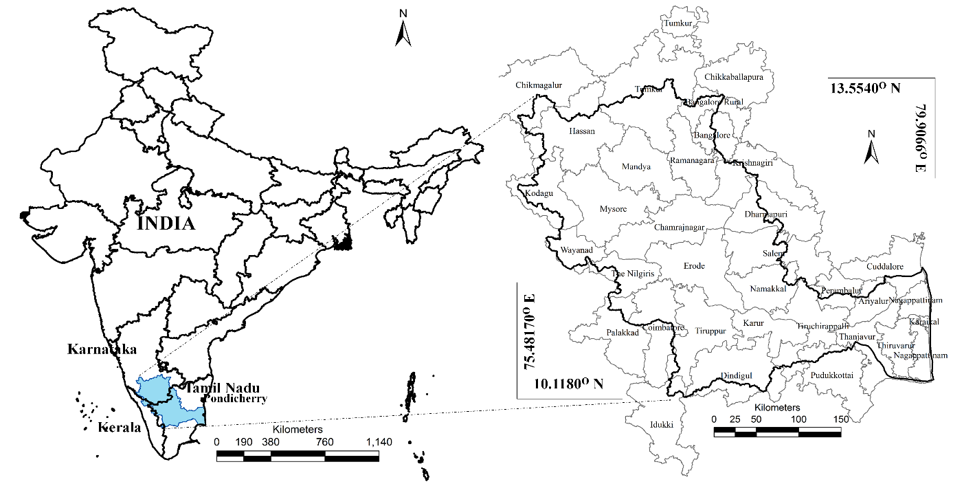
Figure 3.1.3: Administrative division (Districts) with in Cauvery Basin
Table 3.1.2 provides the details of distribution of river Cauvery across the administrative divisions, Cauvery basin has about 55.4% of catchment area spread in Tamil Nadu, followed by Karnataka with 41.1%, Kerala with 3.5%. Cauvery cover nearly 33 districts (Figure 3.1.3) namely i) Bangalore Rural, Bangalore, Chamrajnagar, Chikkaballapura, Chikmagalur, Hassan, Kodagu, Mandya, Mysore, Ramanagara and Tumkur of Karnataka, ii) Idukki, Palakkad and Waynad of Kerala, iii) Ariyalur, Coimbatore, Cuddalore, Dharmapuri, Dindigul, Erode, Karur, Krishnagiri, Nagappattinam, Namakkal, Perambalur, Pudukkottai, Salem, Thanjavur, The Nilgiris, Thiruvarur, Tiruchirappalli, & Tiruppur of Tamil Nadu, iv) Karikal of Puducherry.
As per 2011 Census [7] population in Cauvery basin is about 3,86,55,107 with a density of 452 persons/ sq,km. Figure 3.1.4 and Table 3.1.3 depicts the population dynamics in Cauvery basin and across the administrative boundaries since 1901. Across the administrative boundaries, Tamil Nadu contributes to 58.8% (22732461), followed by Karnataka with 37.9 % (14642518), Kerala with 3.1% (1179200) and Puducherry with 0.35% (100929) of the total population in the basin. Between 1901 and 2011, population has increased from 113 persons per square kilometer to 453 persons per square kilometer. Population growth rate was below 10% per decade until 1941, since then growth rate is over 12% per decade. Highest growth rate was observed between 1961-1971-1981wiht growth rate over 20%. In the recent decade i.e., between 2001 and 2011 population growth is about 14.5% in the basin, Karnataka had highest growth rate of 16.3%, followed by Tamil Nadu with 13.8%, Puducherry with 9.55 and Kerala with 7.6%.
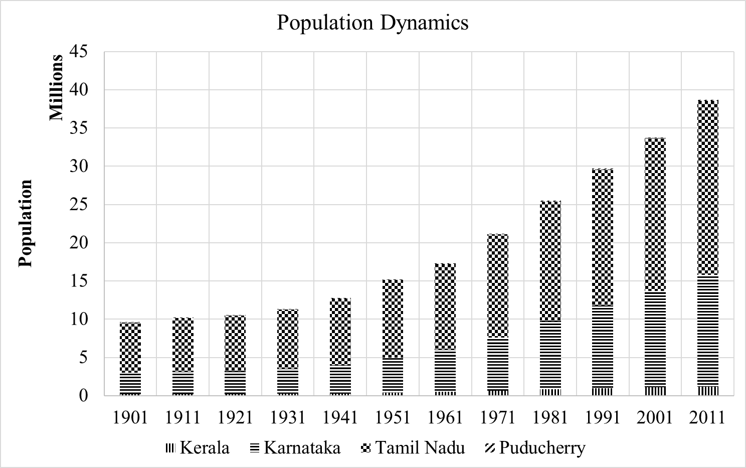
Figure 3.1.4: Population Dynamics in Cauvery River Basin
Table 3.1.3: Population dynamics in Cauvery river basin across administrative divisions
|
Year |
Population Density persons per sq.km |
||||
|
Kerala |
Karnataka |
Tamil Nadu |
Puducherry |
Basin |
|
|
1901 |
65 |
80 |
140 |
252 |
113 |
|
1911 |
70 |
83 |
149 |
265 |
120 |
|
1921 |
72 |
86 |
153 |
259 |
123 |
|
1931 |
81 |
94 |
163 |
267 |
133 |
|
1941 |
93 |
106 |
185 |
286 |
149 |
|
1951 |
124 |
131 |
215 |
332 |
178 |
|
1961 |
165 |
159 |
237 |
366 |
203 |
|
1971 |
222 |
200 |
285 |
426 |
248 |
|
1981 |
283 |
257 |
330 |
488 |
298 |
|
1991 |
336 |
310 |
375 |
550 |
348 |
|
2001 |
383 |
360 |
421 |
598 |
395 |
|
2011 |
409 |
419 |
480 |
655 |
453 |
There are more than 125 Tribal communities in Cauvery basin namely [7]–[9]: Adiyan, Advichincher, Bamcha, Barad, Barodia, Bavacha, Beda, Bedar, Bhagalia, Bhil, Bhil Garasia, Bhilala, Bhine Koya, Burud, Chenchu, Chenchwar, Chodhara, Cholanaickan, Cholivala Nayaka, Dholi Bhil, Dhor Kathodi, Dhor Katkari, Dubla, Dungri Bhil, Dungri Garasia, Eravallan, Gamit, Gamta, Gauriga, Gavit, Gond, Gowdalu, Hakkipikki, Halpati, Haranshikari, Hasaluru, Hill Pulaya, Irular, Irulas, Iruliga, Jeenu Kuruba, Jenu Kurumban, Kaadu Kuruba, Kadar, Kammara , Kanikaran, Kaniyan, Kapadia Nayaka, Karavazhi Pulayan, Karimpalan, Kathodi, Katkari, Kattu Nair, Kattunayakan, Kattunayakas, Kokna, Kokni, Kolcha, Kolgha, Koli Dhor, Konda Kapus, Kondareddis, Konga Malayan , Koraga, Kotas, Kotwalia, Koya, Kudiya, Kukna, Kurichchan, Kurichiyan, Kuruba, Kuruman, Kurumans, Kurumba Pulayan, Kurumba, Kurumban, Maha Malasar, Mala Arayan, Mala Kuruman, Mala Panickar, Malai Arayan, Malai Pandaram, Malai Vedan, Malaikudi, Malakkuravan, Malasar, Malavedan, Malayali , Malayan, Malayarayar, Malayekandi, Maleru, Mannan, Maratha, Marati, Mavchi, Mavilan, Meadar, Meda, Medari, Melakudi, Mewasi Bhil, Mota Nayaka, Mudugar, Muduvan, Mulla Kuruman, Mullu Kuruman, Muthuvan, Naik, Naikda, Naikpod, Nana Nayaka, Nattu Malayan, Nayak, Nayaka, Padvi, Paliyan, Palleyan, Palliyan, Palliyar, Pamba Pulayan, Paniyan, Paniyas, Pardhi, Patelia, Pawra, Phanse Pardhi, Rajgond, Rajkoya, Rathawa, Ravula, Rathwas, Rawal Bhil, Sholaga, Sholiga, Son Kathodi, Son Katkari, Tadvi Bhil, Talavia, Ten Kurumban, Thachanadan, Thachanadan Moopan, Then Kuruba, Toda, Toda , Todas, Tokre Koli, Ulladan, Ullatan, Uraly, Valmiki, Valvi, Vasava, Vasave, Vetta Kuruman, Vitolia, Yerava.
Rainfall[10] in the basin varies between 480 mm at the interior of Karnataka and Tamil Nadu State to 5500mm at the Ghats of Karnataka and Kerala (Figure 3.1.5). Coastal Tamil Nadu receives between 1000mm to 1500mm of rainfall. On an average across the basin, Cauvery receives average rainfall about 950 mm. Catchment receives rains in both in the south west and north east monsoons. Western Ghats receives most of the rainfall between June to September (South West Monsson) whereas the Uplands and Plateau receive rains between August and October and the coasts receiving rainfall between September and December (North East Monsoon). Roughly about 49% of the total precipitation in the catchment is received by South West Monsoons, about 32% by North East Monsoons, and 17% as pre monsoon showers (April and May), during the other months (January, February and March) rainfall is insignificant i.e., about 3% (Figure 3.1.6).

Figure 3.1.5: Rainfall contours across Cauvery river basin
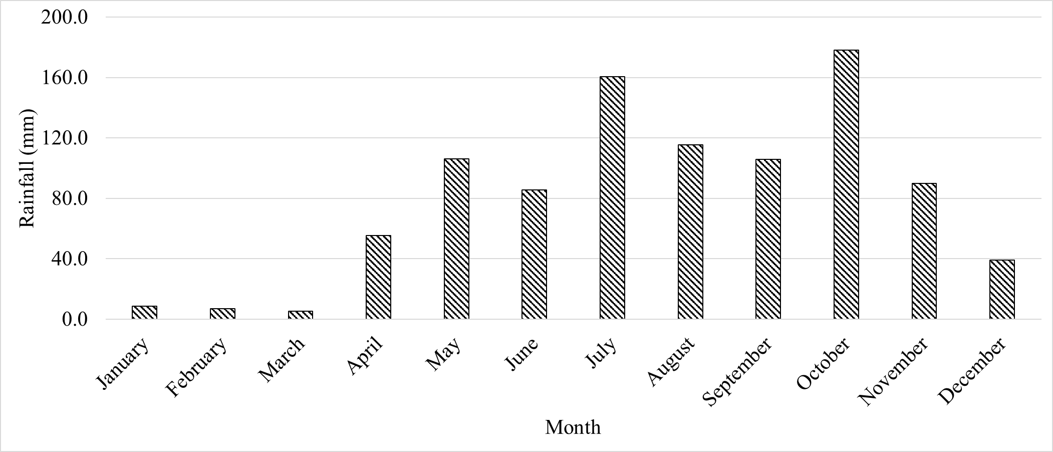
Figure 3.1.6: Rainfall variability throughout the year
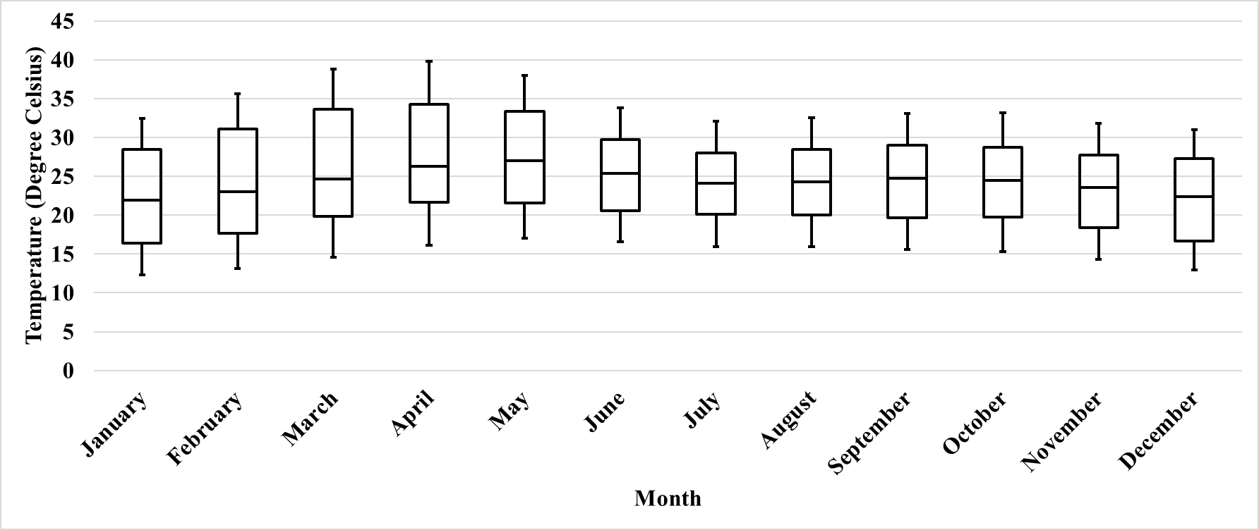
Figure 3.1.7: Monthly temperature variations across the catchment
Temperature: Figure 3.1.7 depicts the temperature variations across the basin [11]. Temperature goes to the trough (minimum) in the months of December and January (as low as 12 degrees Celsius), where as it goes to the crest (maximum) in the months of March and April (as high as 39 degrees Celsius). Across the basin the temperature differences ranges between 8 to 12 degree Celsius. Spatially (Figure 3.1.8), temperature is higher at the East coast (Tamil Nadu), Plains of Tamil Nadu, followed by Plain of Karnataka and lowest at the Western Ghats of Kerala.

Figure 3.1.8: Spatial Temperature vitiations (Average annual temperature)
Agro Ecological and Climatic Zones: Agro-Ecological regions [12] of India can be categorized into 18 physiographic regions such as i) Western Himalayas, ii) Central Himalayas, iii) Eastern Himalayas, iv) North Eastern Hills, v) Western Ghats, vi) Eastern Ghats and Tamil Nadu Uplands, vii) Central Highlands, viii) Eastern Plateau, ix) Deccan Plateau, x) Kachchh and Kathiawar Peninsular, xi) Western Plains, xii) Northern Plains , xiii) Eastern Plains, xiv) Gujarat Plains, xv) Assam and Teesta Valley, xvi) West Coast Plains, xvii) East Coast Plains, xviii) Islands. Cauvery falls under ecological zones of i) Western Ghats, ii) Deccan Plateau, iii) Eastern Ghats and Tamil Nadu uplands, iv) East Coast Plains. Based on climatic characteristics (Figure 3.1.9), Cauvery is dominated by hot semi-arid zone, followed by the Hot Dry Semi-Arid, Hot Moist Semi-Arid and Hot-Moist Sub Humid to Humid Transition Zones. The Western Ghats fall under the category of Hot Moist Semi-Arid and Hot-Moist Sub Humid to Humid Transition Zone, Deccan Plateau of Karnataka and Tamil Nadu Uplands (and Plains) fall under the Hot Semi-Arid Climatic Zone.
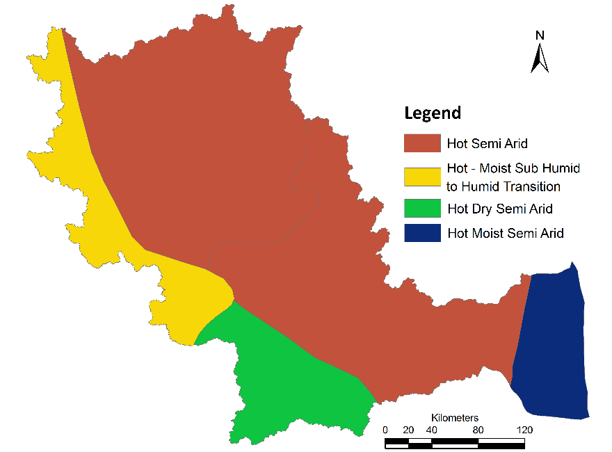
Figure 3.1.9: Agro Climatic Zone of Cauvery Basin
Soil map of India [13] was used to understand soils of Cauvery ( Figures 3.1.10). Soils across India as per their physical properties is classified under 26 categories, of which soils in Cauvery are under 6 categories namely i) Coastal Alluvial, ii) Deltaic Alluvial, iii) Lateritic, iv) Mixed Red and Black Soil, v) Red Loamy & vi) Red Sandy Soils. Red Sandy soil is dominated across the catchment. Table 3.1.5 describes in detail soil type and their locations in Cauvery basin
Table 3.1.5: Soils of Cauvery basin [14]
|
Soil |
Location |
|
Red Loamy |
The Eastern slope of Western Ghats in Karnataka State and upper reaches of the Karnataka basin area around Krishna Raja Sagara & also entire Vrishabhavathi valley south of Mandya |
|
Red Sandy |
Bhavani sub basin of Palghat District in Kerala, Major part of the middle and lower Karnataka basin, Tanjavur, Coimbatore, Nilgiris, Periyar, Dharmapuri, Annamalai, Salem in Tamil Nadu |
|
Laterite |
A small part north west of Mercara, a small part in Wayanad District of Kerala State |
|
Forest Loamy |
Wayanad District -Kabani basin |
|
Loamy Organic |
Coimbatore district - Tamil Nadu |
|
Medium Black Soil |
Idukki District of Kerala State |
|
Reddish Brown |
Thanjavur, Tiruchi, Salem, Periyar, Anna & Coimbatore District. |
|
Black |
Thanjavur & Coimbatore District of Tamil Nadu |
|
Sandy |
South Arcot |
|
Alluvial Clay - Sand |
Extreme south-east corner of the Cauvery basin |

Fig 3.1.10: Soil map of Cauvery
Lithology/Geology: Geological maps of Kerala, Karnataka and Tamil Nadu [15], [16] were used to understand the geology of Cauvery Basin is as depicted in Figure 3.1.11. about 7 lithological forms can be found in the basin namely i) Alluvia, ii) Charnockite, iii) Dharwar, iv) Gneiss, v) Granite, vi) Laterite, vii) Sandstone. Catchment is dominated by Gneisses rocks throughout followed by Alluvia towards the East Coast of Tamil Nadu, Granite in Deccan plateau of Karnataka and Dharwars along the ridges between West to East.
Topography: Elevation and slope maps are as depicted in Figure 3.1.12 and Figure 3.1.13. Shuttle Radar Topographic Mission- SRTM data[17] was used to develop elevation and slope map for the basin. Highest elevation in Western Ghats is at the Annamudi peak (Munnar) in Kerala with elevation about 2695 m AMSL. In the Cauvery basin, highest elevation was at Annamudi hill ranges with elevation about 2629 m AMSL. Followed by Attabppadi hill ranges with elevations up to 2391 m AMSL. Talakaveri i.e., origin of Kaveri river in the Brahmagiri hills is at an elevation of 1341 m. The western Ghats continue from Mettupalyam to Bangalore (diagonally) i.e., the Mysore Elephant Corridor divide the basin to different agro-ecological zones i.e., Deccan Plateau and Uplands. The election drops from about 600 meters, it is also evident from the slope map that the transition zone between Plateau and Uplands have very high slopes.

Figure 3.1.11: Geological Map of Cauvery
Forest: The Cauvery river basin of South India is one of the last global frontiers with diverse endangered and threatened species. Cauvery river basin has naturally endowed with a diversity of bioclimatic, topographic and edaphic variations resulting in rich floristic, wildlife abundance and supporting millions of human kind through profuse natural resources. Cauvery passes eastwards into humid, moist sub-humid, dry sub-humid and semiarid zones and physio-graphically, the basin can be divided into three parts: Western Ghats area, Plateau of Mysore and the Delta, which are responsible for varied forest types across different regions. Forest types found in the basin are tropical evergreen, semi-evergreen, moist and dry deciduous, high altitude sholas, savannas, scrub forests and mangroves. The rich biodiversity with high endemism can be attributed to varied geographical-climatic characteristics. The basin forms an important socio-economic lifeline for major South-India portion harbors numerous elements of flora and fauna having linage to the Gondavana land. The region is rich with the diverse flora and fauna, which are economically and ecologically significant. Due to the incredible biodiversity, basin is also part of Nilgiri bio-sphere reserve.

Figure 3.1.12: Topographic map of Cauvery

Figure 3.1.13: Slope (%) map of Cauvery Basin
Protected Areas:Cauvery river basin has sensitive flora and fauna, realizing its rich ecological values many PAs were created. The PAs are acting as a reserve of diversity and supporting life forms. The uncontrolled anthropogenic disturbances are impacting PAs and its environs. The current study tries to understand status of PAs in Cauvery basin and their ecological status. The Cauvery basin has 26 major PAs covering 3 states supporting numerous biodiversity of various life forms (Figure 3.1.14). Table 3.1.6 provides the details of PAs and their year of establishment and priority for conservation.
Table 3.1.6: PAs of Cauvery basin and their details[18], [19].
|
Sno |
Name |
Designation |
Area km2 |
Established |
State |
Districts |
IUCN Category |
|
1 |
Adichunchanagiri Peacock Sanctuary |
Sanctuary |
0.88 |
1981 |
Karnataka |
Mandya |
Not Reported |
|
2 |
Arabithittu Wildlife Sanctuary |
Sanctuary |
13.5 |
1985 |
Karnataka |
Mysore |
IV |
|
3 |
Bandipur National Park |
National Park |
874.2 |
1974 |
Karnataka |
Mysore, Chamarajanagar |
II |
|
4 |
Bannerghatta National Park |
National Park |
104.27 |
1974 |
Karnataka |
Bangalore, Ramnagara |
II |
|
5 |
Biligiri Ranga Swamy Temple Wildlife Sanctuary |
Sanctuary |
249.6 |
1987 |
Karnataka |
Chamarajanagar |
IV |
|
6 |
Brahmagiri Wildlife Sanctuary |
Sanctuary |
281.0 |
1974 |
Karnataka |
Kodagu |
Not Reported |
|
7 |
Cauvery Wildlife Sanctuary |
Sanctuary |
1027.5 |
1987 |
Karnataka |
Mysore, Bangalore & Mandya |
IV |
|
8 |
Melkote Temple Santuary |
Sanctuary |
49.82 |
1974 |
Karnataka |
Mandya |
IV |
|
9 |
MM HILLS Wildlife Sanctuary |
Sanctuary |
906.19 |
2013 |
Karnataka |
Chamarajanagar |
IV |
|
10 |
Pushpagiri Wildlife Sanctuary |
Sanctuary |
102.92 |
1987 |
Karnataka |
Kodagu & Dakshina Kannada |
IV |
|
11 |
Rajiv Gandhi National Park |
National Park |
643.39 |
1974 |
Karnataka |
Kodagu, Mysore |
II |
|
12 |
Ranganathittu Bird Sanctuary |
Sanctuary |
0.67 |
1940 |
Karnataka |
Mysore |
IV |
|
13 |
Talakaveri Wildlife Sanctuary |
Sanctuary |
105.01 |
1987 |
Karnataka |
Kodagu |
IV |
|
14 |
Anamudi Shola National Park |
National Park |
7.50 |
2003 |
Kerala |
Idukki |
II |
|
15 |
Aralam Wildlife Sanctuary |
Sanctuary |
55.00 |
1984 |
Kerala |
Kannur |
IV |
|
16 |
Chinnar Wildlife Sanctuary |
Sanctuary |
90.44 |
1984 |
Kerala |
Idukki |
IV |
|
17 |
Eravikulam National Park |
National Park |
97.00 |
1978 |
Kerala |
Idukki |
II |
|
18 |
Karimpuzha National Park |
National Park |
225.0 |
2006 |
Kerala |
Palakkad |
Not Reported |
|
19 |
Silent Valley National Park |
National Park |
89.52 |
1984 |
Kerala |
Palakkad |
II |
|
20 |
Wayanad Wildlife Sanctuary |
Sanctuary |
344.44 |
1973 |
Kerala |
Wayanad |
IV |
|
21 |
Anamalai Wildlife Sanctuary |
Sanctuary |
841.49 |
1976 |
Tamil Nadu |
Coimbatore |
IV |
|
22 |
Mudumalai Wildl Life Sanctuary |
Sanctuary |
217.76 |
1942 |
Tamil Nadu |
Nilgiri |
IV |
|
23 |
Mukurthi National Park |
National Park |
78.00 |
2001 |
Tamil Nadu |
Nilgiri |
Not Reported |
|
24 |
Pichavaram Wildl Life Sanctuary |
Sanctuary |
11.00 |
1935 |
Tamil Nadu |
Cuddalore |
Not Reported |
|
25 |
Point Calimere Life Sanctuary |
Sanctuary |
172.6 |
1967 |
Tamil Nadu |
Nagapattinam |
IV |
|
26 |
Satyamangalam Wildlife Sanctuary |
Sanctuary |
1408.5 |
2011 |
Tamil Nadu |
Erode |
II |
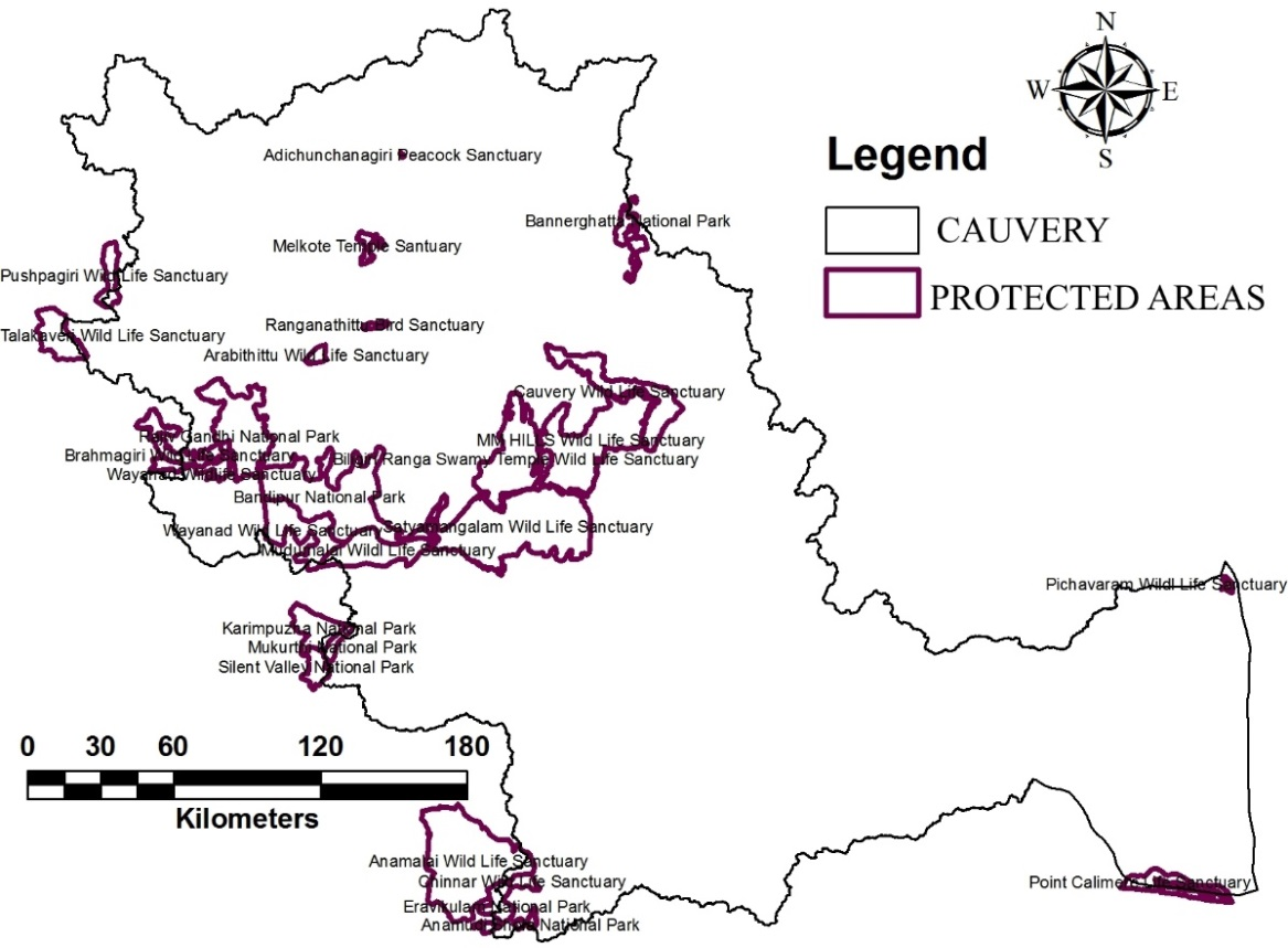
Figure 3.1.14: PAs of Cauvery basin
Reservoirs: In India, soon after independence Dams and Reservoirs were treated as temples of development with no/very little consult and comply to meet the needs of user community [20]. The reservoirs and dams are often viewed as i) Hydro power generators, ii) Flood mitigation units, iii) Source of Drinking water supply, iv) Water Containers [21]. River Cauvery consists one of the oldest living dam in the world having an history over 1800 years, built in 2nd century AD, i.e., The Grand Anicut (Kallanai Dam), built by King Karikalan of the Chola dynasty for irrigating alluvial delta (Tanjavore) of Cauvery [22]. Water Resource Information System [2] records about 98 major and minor irrigation dams and numerous lakes in the Cauvery Basin. Reservoir in the basin have a live storage capacity of 297 TMC and gross storage capacity of 329 TMC. Figure 3.1.15 and Table 3.1.7 describes in detail dams and their capacities. Karnataka has 57 dams with gross storage capacity of 157 TMC and live storage of 133 TMC, Tamil Nadu has 37 dams with gross storage capacity of 160 TMC and live storage of 154 TMC, Kerala has 4 dams with gross storage of 13 TMC and live storage of 10 TMC. Of all the Dams, Mettur dam (Stanley Reservoir) has highest storage capacity of capacity 95.6 TMC (93.4 TMC), followed by Krishnaraja Sagara Dam with capacity of 49.44 TMC (45.1 TMC), Hemavathi with 37.1 TMC (32.7 TMC), Lower Bhavani with 32.8 TMC (32.1 TMC), Kabini with 19.5 TMC (16 TMC), Siruvani with 9 TMC (6.5 TMC), Harangi with 8.5 TMC (8.1 TMC) capacity. Other dams have capacities lower than 8 TMC.
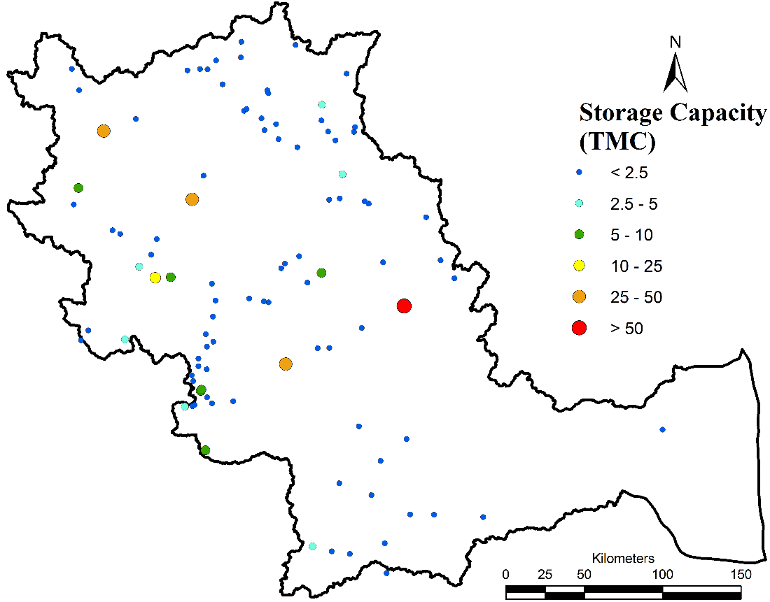
Figure 3.1.15: Reservoirs in Cauvery River Basin
Table 3.1.7: Reservoirs in Cauvery river Basin
|
Sl.no |
Reservoir |
Latitude |
Longitude |
State |
Gross Storage |
Live Storage |
||
|
Kilo.cum |
TMC |
Kilo.cum |
TMC |
|||||
|
1 |
Krishnarajasagar Dam |
12.43 |
76.57 |
Karnataka |
1400000 |
49.441 |
1275690 |
45.051 |
|
2 |
Hemavathy Dam |
12.82 |
76.05 |
Karnataka |
1050630 |
37.103 |
926830 |
32.731 |
|
3 |
Kabini Dam |
11.97 |
76.35 |
Karnataka |
552740 |
19.520 |
453065 |
16.000 |
|
4 |
Harangi Dam |
12.49 |
75.91 |
Karnataka |
240690 |
8.500 |
228560 |
8.072 |
|
5 |
Uduthorehalla Dam |
12.00 |
77.33 |
Karnataka |
189972 |
6.709 |
151509 |
5.535 |
|
6 |
Nugu Dam |
11.98 |
76.44 |
Karnataka |
154042 |
5.440 |
129850 |
4.586 |
|
7 |
Taraka Dam |
12.04 |
76.26 |
Karnataka |
111567 |
3.940 |
90754 |
3.205 |
|
8 |
Tippagondana Hally Dam |
12.97 |
77.34 |
Karnataka |
94719 |
3.345 |
19713 |
0.696 |
|
9 |
Maralvadi Dam |
12.56 |
77.46 |
Karnataka |
74040 |
2.615 |
67350 |
2.378 |
|
10 |
Marconahally Dam |
12.93 |
76.88 |
Karnataka |
68000 |
2.401 |
64000 |
2.260 |
|
11 |
Arkavathy Dam |
12.42 |
77.44 |
Karnataka |
44940 |
1.587 |
40493 |
1.430 |
|
12 |
Votehole Dam |
13.06 |
75.91 |
Karnataka |
42758 |
1.510 |
38680 |
1.366 |
|
13 |
Suvarnavathy Dam |
11.83 |
77.02 |
Karnataka |
35679 |
1.260 |
35650 |
1.259 |
|
14 |
Manchanabele Dam |
12.87 |
77.34 |
Karnataka |
34603 |
1.222 |
30044 |
1.061 |
|
15 |
Hesaraghatta Dam |
13.14 |
77.49 |
Karnataka |
29591 |
1.045 |
114 |
0.004 |
|
16 |
Gundal Dam |
12.09 |
77.20 |
Karnataka |
27439 |
0.969 |
23220 |
0.820 |
|
17 |
Byramangala Dam |
12.76 |
77.42 |
Karnataka |
24100 |
0.851 |
22010 |
0.777 |
|
18 |
Kanva Dam |
12.72 |
77.19 |
Karnataka |
23880 |
0.843 |
22710 |
0.802 |
|
19 |
Mallaghatta Dam |
13.18 |
76.62 |
Karnataka |
16620 |
0.587 |
14860 |
0.525 |
|
20 |
Kadaba Dam |
13.24 |
76.87 |
Karnataka |
16530 |
0.584 |
15700 |
0.554 |
|
21 |
Kunigal Dodakere Dam |
13.03 |
77.03 |
Karnataka |
15070 |
0.532 |
13700 |
0.484 |
|
22 |
Mangala I Dam |
12.94 |
76.90 |
Karnataka |
15000 |
0.530 |
13500 |
0.477 |
|
23 |
Thonnur Dam |
12.56 |
76.64 |
Karnataka |
13660 |
0.482 |
12420 |
0.439 |
|
24 |
Kodaganar Dam |
13.05 |
77.02 |
Karnataka |
12300 |
0.434 |
11540 |
0.408 |
|
25 |
Deepambudikere Dam |
12.86 |
77.07 |
Karnataka |
12106 |
0.428 |
9687 |
0.342 |
|
26 |
Hebbahalla Dam |
12.11 |
76.33 |
Karnataka |
11978 |
0.423 |
8190 |
0.289 |
|
27 |
Chickkahole Dam |
11.83 |
76.99 |
Karnataka |
10648 |
0.376 |
10534 |
0.372 |
|
28 |
Maidal Amanikere Dam |
13.31 |
77.19 |
Karnataka |
7400 |
0.261 |
6970 |
0.246 |
|
29 |
Muthurayanakere Dam |
12.82 |
77.00 |
Karnataka |
6795 |
0.240 |
5872 |
0.207 |
|
30 |
Nidasale Dam |
12.77 |
77.08 |
Karnataka |
6632 |
0.234 |
5306 |
0.187 |
|
31 |
Nallur Amanikere Dam |
11.84 |
76.71 |
Karnataka |
6541 |
0.231 |
5890 |
0.208 |
|
32 |
Nelligudda Dam |
12.81 |
77.37 |
Karnataka |
6130 |
0.216 |
5680 |
0.201 |
|
33 |
Chikkagondanahally Dam |
12.41 |
77.59 |
Karnataka |
5900 |
0.208 |
2463 |
0.087 |
|
34 |
Mangala II Dam |
11.65 |
76.65 |
Karnataka |
5850 |
0.207 |
4890 |
0.173 |
|
35 |
Kachavanahalli Dam |
12.23 |
76.15 |
Karnataka |
5740 |
0.203 |
5100 |
0.180 |
|
36 |
Nittur Dam |
13.33 |
76.87 |
Karnataka |
5410 |
0.191 |
5410 |
0.191 |
|
37 |
K.Honnamachanahalli Dam |
12.89 |
76.98 |
Karnataka |
5210 |
0.184 |
4750 |
0.168 |
|
38 |
Chiklihole Dam |
12.40 |
75.88 |
Karnataka |
5097 |
0.180 |
4729 |
0.167 |
|
39 |
Turuvekere Dam |
13.17 |
76.67 |
Karnataka |
5070 |
0.179 |
4870 |
0.172 |
|
40 |
Mayasandra Dam |
13.09 |
76.76 |
Karnataka |
4860 |
0.172 |
3885 |
0.137 |
|
41 |
Obichudanahally Dam |
12.81 |
77.53 |
Karnataka |
4670 |
0.165 |
3300 |
0.117 |
|
42 |
Doddaladahalli Dam |
12.42 |
77.38 |
Karnataka |
4353 |
0.154 |
3190 |
0.113 |
|
43 |
Sarigehally Dam |
13.23 |
76.72 |
Karnataka |
4300 |
0.152 |
4300 |
0.152 |
|
44 |
Chakena Hally Dam |
12.89 |
76.24 |
Karnataka |
4280 |
0.151 |
3920 |
0.138 |
|
45 |
Hosahalli Dam |
12.02 |
77.09 |
Karnataka |
3240 |
0.114 |
2940 |
0.104 |
|
46 |
Kalikatte Dam |
11.75 |
76.69 |
Karnataka |
3170 |
0.112 |
2720 |
0.096 |
|
47 |
Kamarahalli Dam |
11.94 |
76.69 |
Karnataka |
2960 |
0.105 |
2540 |
0.090 |
|
48 |
Gowdahally Dam |
12.05 |
77.11 |
Karnataka |
2390 |
0.084 |
2230 |
0.079 |
|
49 |
Gopinatham Dam |
12.05 |
77.69 |
Karnataka |
2180 |
0.077 |
1900 |
0.067 |
|
50 |
Alaluru Dam |
12.25 |
76.10 |
Karnataka |
2180 |
0.077 |
2070 |
0.073 |
|
51 |
New Amachawadi Dam |
11.85 |
76.90 |
Karnataka |
1690 |
0.060 |
1560 |
0.055 |
|
52 |
Kowlihalla Dam |
11.94 |
77.25 |
Karnataka |
550 |
0.019 |
490 |
0.017 |
|
53 |
Karimuddenahalli Dam |
12.20 |
76.36 |
Karnataka |
180 |
0.006 |
179 |
0.006 |
|
54 |
Yagachi Dam |
13.18 |
75.87 |
Karnataka |
90 |
0.003 |
80782 |
2.853 |
|
55 |
Neralatti Kere Dam |
12.39 |
77.61 |
Karnataka |
|
|
|
|
|
56 |
Kuppareddy Dam |
12.84 |
77.53 |
Karnataka |
|
|
|
|
|
57 |
Nonavinakere Lake Dam |
13.17 |
76.55 |
Karnataka |
|
|
|
|
|
58 |
Siruvani( I D) Dam |
10.98 |
76.64 |
Kerala |
255000 |
9.005 |
184200 |
6.505 |
|
59 |
Karapuzha (Id) Dam |
11.62 |
76.17 |
Kerala |
76500 |
2.702 |
72000 |
2.543 |
|
60 |
Kuttiyadi Spillway Dam |
11.67 |
75.96 |
Kerala |
38400 |
1.356 |
33980 |
1.200 |
|
61 |
Near Kottagiri Saddle Dam |
11.61 |
75.92 |
Kerala |
|
|
|
|
|
62 |
Mettur Dam |
11.80 |
77.81 |
Tamil Nadu |
2707128 |
95.601 |
2645201 |
93.414 |
|
63 |
Lower Bhavani Dam |
11.47 |
77.11 |
Tamil Nadu |
929000 |
32.807 |
908000 |
32.066 |
|
64 |
Avalanche lake |
11.32 |
76.62 |
Tamil Nadu |
156200 |
5.516 |
152800 |
5.396 |
|
65 |
Emerald Lake |
11.33 |
76.62 |
Tamil Nadu |
156200 |
5.516 |
152800 |
5.396 |
|
66 |
Amaravathi reservoir |
10.42 |
77.26 |
Tamil Nadu |
114600 |
4.047 |
109360 |
3.862 |
|
67 |
Upper Bhavani Dam |
11.23 |
76.52 |
Tamil Nadu |
101200 |
3.574 |
85200 |
3.009 |
|
68 |
Pykara Dam |
11.46 |
76.60 |
Tamil Nadu |
56630 |
2.000 |
55080 |
1.945 |
|
69 |
Mukurthy Dam |
11.41 |
76.56 |
Tamil Nadu |
50980 |
1.800 |
50710 |
1.791 |
|
70 |
Pillur Dam |
11.26 |
76.81 |
Tamil Nadu |
44400 |
1.568 |
34970 |
1.235 |
|
71 |
Palar Porundalar Dam |
10.37 |
77.48 |
Tamil Nadu |
43130 |
1.523 |
43130 |
1.523 |
|
72 |
Sandy nalla dam |
11.44 |
76.65 |
Tamil Nadu |
26620 |
0.940 |
2310 |
0.082 |
|
73 |
Noyyal Orathupalayam Dam |
11.11 |
77.54 |
Tamil Nadu |
17440 |
0.616 |
17440 |
0.616 |
|
74 |
Uppar( Erode) Dam |
10.78 |
77.42 |
Tamil Nadu |
16310 |
0.576 |
14920 |
0.527 |
|
75 |
Kodaganar Dam |
10.59 |
77.97 |
Tamil Nadu |
12300 |
0.434 |
11540 |
0.408 |
|
76 |
Thoppaiyar Dam |
11.96 |
78.11 |
Tamil Nadu |
8433 |
0.298 |
8433 |
0.298 |
|
77 |
Vattamalaikarai Odai Dam |
10.91 |
77.66 |
Tamil Nadu |
7590 |
0.268 |
6890 |
0.243 |
|
78 |
Kuthiraiyar Dam |
10.39 |
77.38 |
Tamil Nadu |
7200 |
0.254 |
7200 |
0.254 |
|
79 |
Nanganjiyar Dam |
10.60 |
77.83 |
Tamil Nadu |
7200 |
0.254 |
6590 |
0.233 |
|
80 |
Gunderipallam Dam |
11.56 |
77.37 |
Tamil Nadu |
7200 |
0.254 |
7200 |
0.254 |
|
81 |
Noyyal Athupalayam Dam |
11.03 |
77.82 |
Tamil Nadu |
6600 |
0.233 |
6430 |
0.227 |
|
82 |
Siddhamalli Dam |
11.07 |
79.31 |
Tamil Nadu |
6418 |
0.227 |
6418 |
0.227 |
|
83 |
Nallathangal Odai Dam |
10.71 |
77.61 |
Tamil Nadu |
6330 |
0.224 |
6330 |
0.224 |
|
84 |
Parappalar Dam |
10.43 |
77.68 |
Tamil Nadu |
5600 |
0.198 |
5600 |
0.198 |
|
85 |
Nagavathi Dam |
12.06 |
78.03 |
Tamil Nadu |
4650 |
0.164 |
4387 |
0.155 |
|
86 |
Varattupallam Dam |
11.68 |
77.56 |
Tamil Nadu |
3950 |
0.139 |
3910 |
0.138 |
|
87 |
Kesarigulihalla Dam |
12.31 |
77.95 |
Tamil Nadu |
3795 |
0.134 |
3566 |
0.126 |
|
88 |
Ponnaniar Dam |
10.58 |
78.26 |
Tamil Nadu |
3396 |
0.120 |
3396 |
0.120 |
|
89 |
Perumpallam Dam |
11.56 |
77.30 |
Tamil Nadu |
3280 |
0.116 |
3180 |
0.112 |
|
90 |
Kundah Palam Dam |
11.28 |
76.65 |
Tamil Nadu |
1760 |
0.062 |
1560 |
0.055 |
|
91 |
West Varahapallam Weir Dam |
11.23 |
76.57 |
Tamil Nadu |
1360 |
0.048 |
|
|
|
92 |
Pegumbahallah Forebay Dam |
11.25 |
76.68 |
Tamil Nadu |
1070 |
0.038 |
1030 |
0.036 |
|
93 |
Glemorgan Dam |
11.51 |
76.60 |
Tamil Nadu |
740 |
0.026 |
|
|
|
94 |
East Varahapallam dam |
11.24 |
76.58 |
Tamil Nadu |
400 |
0.014 |
|
|
|
95 |
Moyar Forebay Dam |
11.60 |
76.69 |
Tamil Nadu |
170 |
0.006 |
170 |
0.006 |
|
96 |
Porthimund Dam |
11.38 |
76.57 |
Tamil Nadu |
126 |
0.004 |
123 |
0.004 |
|
97 |
Marudhanadi Dam |
10.26 |
77.69 |
Tamil Nadu |
|
|
|
|
|
98 |
Maravakandi Forbay Dam |
11.57 |
76.65 |
Tamil Nadu |
|
|
|
|
IRRIGATION
River Cauvery has one of the oldest irrigation practices in the history aging over to the Sangam Period 300 BC, during the era people knew type of soil and what kind of crops that can be grown accordingly [23], [24]. Some of the ancient remain based on the archeological surveys indicate the irrigation practices of paddy cultivation goes beyond 1000 BC [24], [25]. Tamil Sangam poems describe ancient understanding of paddy and its utilization[24].
நறுங்காழ்கொன்று, கோட்டின்வித்திய
குறுங்கதிர்த்தோரை, நெடுங்கால்ஐயவி,
ஐவனவெண்ணெலொடுஅரில்கொள்புநீடி; (Madurai kanji 288)
Madurai Kanji explains about Ivvanamnel variety of paddy in the hilly zones along with Ven-Nel.
பைதுஅறவிளைந்தபெருஞ்செந்நெல்லின் (Perumban attrupadai-230)
Perumbanattrupadai explains paddy physiology, the native people’s understanding in harvesting and their understanding of suitable stage of Paddy variety for harvesting
கூனி, குயத்தின்வாய்நெல்அரிந்து,
சூடுகோடாகப்பிறக்கி, நாள்தொறும்,
குன்றுஎனக்குவைஇயகுன்றாக்குப்பை
கடுந்தெற்றுமூடையின்இடம்கெடக்கிடக்கும்,
சாலிநெல்லின், சிறைகொள்வேலி,
ஆயிரம்விளையுட்டுஆக,
காவிரிபுரக்கும்நாடுகிழவோனே. (Porunnarattrupadai -240-45)
Porunnarattrupadai -240-45: Matured paddy which is about to ready for harvest and talks about pumper yield of rice - aayiramveli (it is definitely a very high yield, the quantitative unit veli to be studied. – Aayiram- one thousand
உணவுகொடுத்துஓம்பியமுறை
முரவைபோகியமுரியாஅரிசி
விரல்எனநிமிர்ந்தநிரல்அமைபுழுக்கல்,
பரல்வறைக்கருனை, காடியின்மிதப்ப( PorunnarAttrupadai 105-115)
PorunnarAttrupadai 105-115 narrates cooking methods and the selection of rice that is unbroken rice from the par boiled long grain
அரிசெத்துஉணங்கியபெருஞ்செந்நெல்லின்
தெரிகொள்அரிசித்திரள்நெடும்புழுக்கல்,
அருங்கடித்தீம்சுவைஅமுதொடு, பிறவும்,
விருப்புடைமரபின்கரப்புடைஅடிசில்,
மீன்பூத்தன்னவான்கலம்பரப்பி, ( PerumbanAttrupadai 475)
PerumbanAttrupadai 475: This poem narrates harvest, post-harvest, drying par boiling techniques, milling at a sequence. This poem represents their paddy processing and usage techniques from Sangam literature.
Since agriculture was rainfall dependent, river was not perennial, many rulers, dug numerous tanks (Gangaikondan Tank, Ponneri Tank, Kaveripakkam Tank, Maduranthakam tank, and may more), constructed semicircular bunds indicating that the people were aware of rain water harvesting [23], [26].
Cholas were the first to understand importance of irrigation and constructed numerous interconnected lakes/tanks/reservoirs making the dry lands as cultivable through artificial irrigation [27]. The tanks not only catered water for domestic needs and irrigation, but also recharge groundwater, mitigate floods. World First irrigation dam built by Cholas in the 2nd Century AD [26], which is still functional as any modern hydraulic structure. The dam was constructed to control the flood waters of Cauvery and irrigate the fertile delta. Due to which Thanjore is said as the Rice Bowl of South India. Crops such as paddy, millets, sugarcane, banana, cardamom, pepper, cotton, sesame, coconut, plantains, sandalwood, tamarind, beans were grown. Crop rotation was in practice black grams were cultivated after paddy which helps in nitrogen fixation. Mixed cropping was also practiced such as growing ginger, turmeric in plantations, millets grown with cotton. The lands were immediately ploughed after harvest so as to allow water to fill to the root zone and help in removing of leftover stocks/roots [23]. The ancient practices of irrigation have made delta the rice bowl of south India.
The constrains raised due to escalation of labor, water, energy have made farming community swapping to alternative and efficient techniques of irrigation. Drip irrigation and sprinkler irrigation received considerable attention from policy makers due to their significant contribution towards resource saving, enhanced agricultural productivity [28]. The drip irrigation refers to providing the irrigation to the root zone of plants through a network of pipes, drippers and emitters that are designed to discharge water at prescribed rates. The sprinkler irrigation system, water is sprinkled under pressure in the form of rainfall over the foliage through nozzles fitted with the network of pipes. The sprinkler is suitable where the cropping density is very high and the drip irrigation is not economical. Recognizing the importance of micro irrigation in economical use of water, both the state and central government have sought to promote micro irrigation through various incentives. The micro irrigation has also emerged as a suitable solution to manage the fast depleting ground water. Earlier studies have documented water savings of 30% to 69 % in various crops and labor savings of 21 to 42 man days/hectare. Similarly, savings in energy and water were estimated over 7 years (2003-04 to 2009-10) to be of the order of 324 mi Kwh and 120 TMC. There was significant impact on income with increased productivity, uniform growth, and earlier maturity [29]. Micro Irrigation through drip and sprinkled technologies are brought under Centrally Sponsored Scheme with the objective to enhance water use efficiency in the agriculture sector by promoting appropriate technological interventions, water saving and conservation. The scheme was launched by the Department of Agriculture & Cooperation, Ministry of Agriculture in January, 2006 as Centrally Sponsored Scheme on Micro Irrigation (CSS). Currently the scheme is under Pradhan Mantri Krishi Sinchayee Yojana (PMKSY). The funding pattern between Central Government and State Government is 50:50%. Table X provides area brought under micro irrigation sachems and their fund allocations. Total area covered under drip irrigation in India is 3371597 Ha and 4357215 Ha under sprinkler irrigation totaling 7728812 Ha under micro irrigation system.
|
S. No. |
State |
Drip |
Sprinkler |
Total |
Fund Allocation in Crores (2015-2016) |
|
1 |
Karnataka |
429903 |
417005 |
846907 |
111 |
|
2 |
Kerala |
22516 |
6948 |
29464 |
5 |
|
3 |
Tamil Nadu |
290009 |
30436 |
320445 |
72.75 |
|
Grand Total |
742428 |
454389 |
1196816 |
188.75 |
|
BIRTH OF RIVER CAUVERY
Geologically, formation of Western Ghats is earlier than the Himalayas [30–34], indicating that Cauvery is ancient than the Ganges. Cauvery Basin is a peri-cratonic basin [35], Isotopic palaeo temperature data suggests south India and Madagascar were located apparently in middle latitudes[36]. Evolution of the Cauvery Basin and subsequent sedimentation along eastern passive margin of India is attributed to the fragmentation of eastern Gondwana and opening up of the Indian Ocean which began in Late Jurassic - Early Cretaceous[37] (Figure 3.1.16). Cretaceous Paleogene sections of the Cauvery Basin are closely related to the rifting and drifting phases of peninsular India[35]. Uplift and eastward tilting of the basin can be linked to the rise of reunion hot spot which caused Deccan volcanic activity in central India[38], this tectonic activity has led to ~ 80m fall in sea level. Figure 3.1.17 depicts the linkage between geological events and their relationships in Cauvery basin
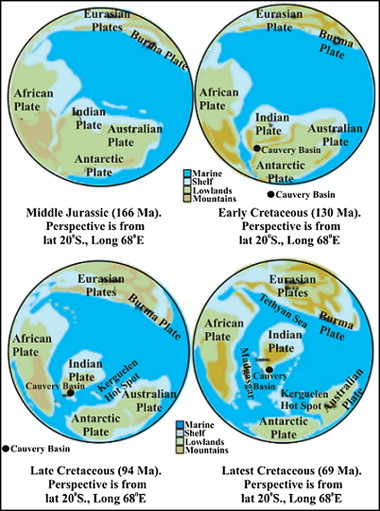
Figure 3.1.16: Paleogeographic maps; shows the Cauvery Basin(Source:[37], [39])
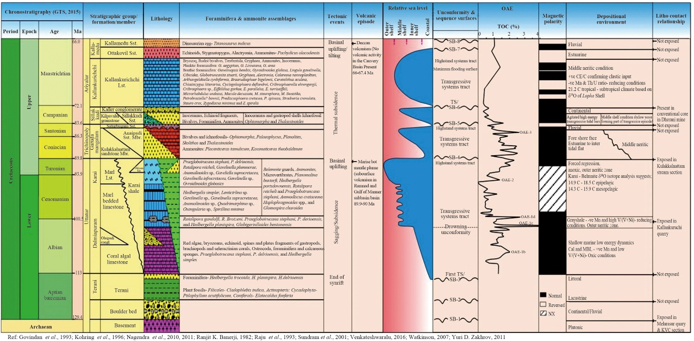
Figure 3.1.17: Geological events in Cauvery Basin, southern India (Source:[35])
Mythologically, Kaveri Purana of Skanda purana (Chapters 11 – 14) describes the birth of river Cauvery[40]. The story of Kaveri goes back to the times of Saudra Mantha i.e., churning of oceans. During the Samudra Mantahana, various objects arrived from ocean, one of which is the nectar of immorality (Amrutha), lord Vishnu forms the avatar of Mohini and Lopmudra (Vishnumaya) was sent by Goddess Lakshmi to aid Mohini to avert demons and bring elixir of life to the Gods. After this, Lopamudra was adopted by Lord Brahma as his daughter. Little later, Sage Kavera went to Brahmagiri hills and prayed to Lord Brahma to bless with offspring. Lord Brahma blessed sage Kavera with Lopamudra. From then after Lopamudra daughter of sage Kavera was known as Kaveri. Kaveri was extremely passionate that her father had all the pleasure and wealth in life and a consecrated terrain full of Nobel and blissful natives. So she departed to Brahmagiri and prayed lord Brahma to turn her into river so she can help people, make land fertile and productive. Brahma approved the boon saying that it would happen in short time. One day while sage Agastya was traveling down south saw Kaveri and fell in love with her. Sage Agastya requested Kaveri to marry. Kaveri agrees for marriage on a condition that Sage Agastya should not leave her alone. Sage Agastya remains true to his promise for several years. Reluctant or leave Cauvery alone, Sage Agastya turns her into water and places in the sacred pot (kamandala). Sage Agastya places the kamandala on the rock and starts meditation. During this time, the Gods decide to release Kaveri to help the people down south. Lord Ganesh in the form of crow knocks down the kamadala releasing Kaveri to flow as a river [40]–[43].
CAUVERY IN ANCIENT LITERATURES
Bhramhanda purana one of the ancient puranas talks about river Cauvery as below [44]
|| ಕಾವೇರೀ ಪ್ರಾರ್ಥನಾ ||
ಮರುದ್ಧೃತೇ ಮಹಾಭಾಗೇ ಮಹಾದೇವಿ ಮನೋಹರೇ
|
ಸರ್ವಾಭೀಷ್ಟಪ್ರದೇ ದೇವಿ ಸ್ನಾಸ್ಥಿತಾಂ ಪುಣ್ಯವರ್ಧಿನಿ ||೧||
ಸರ್ವಪಾಪಕ್ಷಯಕರೇ ಮಮ ಪಾಪಂ
ವಿನಾಶಯ |
ಕಾವೇರಕನ್ಯೇ ಕಾವೇರಿ ಸಮುದ್ರಮಹಿಷಿಪ್ರಿಯೇ ||೨||
ದೇಹಿಮೇ ಭಕ್ತಿಮುಕ್ತಿತ್ವಂ
ಸರ್ವತೀರ್ಥಸ್ವರೂಪಿಣಿ |
ಸಿಂಧುವರ್ಯೆ ದಯಾಸಿಂಧೋ ಮಾಮುದ್ಧರ ದಯಾಂಬುಧೇ
||೩||
ಸ್ತಿçಯಂ ದೇಹಿ ಸುತಂ ದೇಹಿ ಶ್ರಿಯಂ ದೇಹಿ ತತಃ ಸ್ವಗಾ |
ಆಯುಷ್ಯಂ ದೇಹಿ
ಚಾರೋಗ್ಯಂ ಋಣಾನ್ಮುಕ್ತಂ ಕುರುಷ್ವಮಾಮ್ ||೪||
ತಾಸಾಂಚ ಸರಿತಾಂ ಮಧ್ಯೇ ಸಹ್ಯಕನ್ಯಾಘನಾಶಿನಿ
|
ಕಾವೇರಿ ಲೋಕವಿಖ್ಯಾತಾ ಜನತಾಪನಿವಾರಿಣಿ ||೫||
ಇತೀ ಬ್ರಹ್ಮಾಂಡ ಪುರಾಣೇ ಕಾವೇರೀ
ಪ್ರಾರ್ಥನಾ||
Srimad Bhagavatam 11.5.38-40 [45][46] also talks about river Cauvery as holy river in the south India (Dravida desa) during the Kali yug.
ಕ್ರಟದಿಸು ಪ್ರಜಾ ರಾಜನ್
ಕಾಲವ್ ಇಚ್ಚಂತಿ ಸಂಭವA
ಕಾಲೌ ಖಾಲು
ಭವಿಶ್ಯಾಂತಿ
ನಾರಾಯಣ-ಪರಾಯಣಾಃ
ಕ್ವಚಿತ್ ಕ್ವಚಿನ್ ಮಹಾ-ರಾಜ
ದ್ರಾವಿಡೇಸು ಕ ಭೂರಿಸಾಃ
ತಾರ್ಮಪರ್ನಿ ನಾಡಿ ಯಾತ್ರ
ಕ್ರತಾಮಲ ಪಾಯಸ್ವಿನಿ
ಕಾವೇರಿ ಕ
ಮಹಾ-ಪುಣ್ಯಾ
ಪ್ರತೀಸೀ ಕ ಮಹಾ-ನದಿ
ಯೆ ಪಿಬಂತಿ ಜಲಂ ತಾಸಾಂ
ಮನುಜಾ ಮನುಜೆಶ್ವರ
ಪ್ರಾಯೊ ಭಕ್ತಾ
ಭಗವತಿ
ವಾಸುದೆವೆ ಮಲಾಸಯಾಃ
Meaning[46]: My dear King, the inhabitants of Satya-yuga and other ages eagerly desire to
take birth in this Age of Kali, since in this age there will be many devotees of the
Supreme Lord, Narayana. These devotees will appear in various places but will be
especially numerous in South India. O master of men, in the Age of Kali those persons
who drink the waters of the holy rivers of Dravida-desa, such as the Tamraparni,
Krtamala, Payasvini, the extremely pious Kaveri and the Pratici Mahanadi, will almost
all be pure hearted devotees of the Supreme Personality of Godhead,
Vasudeva.
Greatness of Cauvery is stated in ancient literatures such as Agneya
Purana, Mahabharatha,[47]
Agneya Purana
- Kaveri Mahatmyam states,
ಶಟ್ಶಷ್ಠಿ ಕೋಟಿ ತೀರ್ಥಾನಿ ದ್ವಿಸಪ್ತ ಭುವನೇಶು ಚ
Meaning [47]: Sixtysix crores of sacred waters in all the fourteen worlds, come stay in Cauvery, in the month of Thula by the order of Lord Keshava.
ಕೇಶವಸ್ಯ ಆಜ್ಞೇಯ ಯಾಂತಿ ತುಲಾಮಾಸೆ ಮರುದ್ವಿಧಂ - Cauvery river is very important for sri vaishnavas because association with Ranganatha in Adi, Madhya and Anthya ranga kshetraas.
- Punya cannot be obtained without straining the body. Therefore, one who would bathe in the Cauvery should observe these restraints. Bathing without observing the rules will only remove superficial dirt. The body is like a bubble, and is the abode of much filth. Yama is alert, always watchful for loopholes. Morning and evening are enemies which wear away life. Therefore, you should not, you should not, you should not, waste the day. The body is in your command; the senses are not bad. Rivers are easily accessible, and afford sanctity. Autumn is an auspicious season. The man who fears naraka should drive away the demon of sleep, awake at daybreak, and bathe in the waters of the Cauvery. Cauvery, best of rivers, flows incessantly, capable of destroying all sins. Those who bathe in it, without worldly desires, will attain Heaven by mere bathing.
- If Shesha, with big thousand mouths, spoke for 10,000 years, he could not finish recounting the glory of the Cauvery
Mahabharatha declares that i) Ganga can purify a person in 3 nights, ii) Krishnaveni in 4 days, iii) Yamuna in 5 nights, iv) Hemakoota in 5 nights, v) Goutamee in 5 nights, vi) Tunga in 10 nights, vii) Carvery can purify immediately even the prosperities sins till death.
Puranas affirm that there are five means of wiping out the five
capital sins and attaining salvation i) the urusha-Sookta among the Vedas, ii) the Geeta
in the Mahabharata, iii) the Gayatri among mantras, iv) Ekadasi among Vratas, v) among
river-baths, bathing in the Cauvery in the month of Tula (Aippisi), in the presence of
Ranganatha.
Valmiki Ramayana [48] in Kishkindha Kanda 4-41-14 also indicates
Cauvery as a divine river where in Apsaras would be making their pleasure trips
ತಥಾ ತಾಂ ಆಪಗಾಂ ದಿವ್ಯಾಂ ಪ್ರಸನ್ನ ಸಲಿಲಾಶಯಾನ್ || ೪-೪೧-೧೪
ತತ್ರ
ದ್ರಕ್ಷö್ಯಥ ಕಾವೆರೀಂ ವಿಹರಿತಾಂ ಅಪ್ಸರೊ ಗಣೈಹಿ|
LANDSCAPE ELEMENTS OF CAUVERY RIVER BASIN
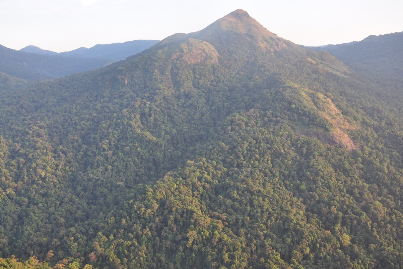
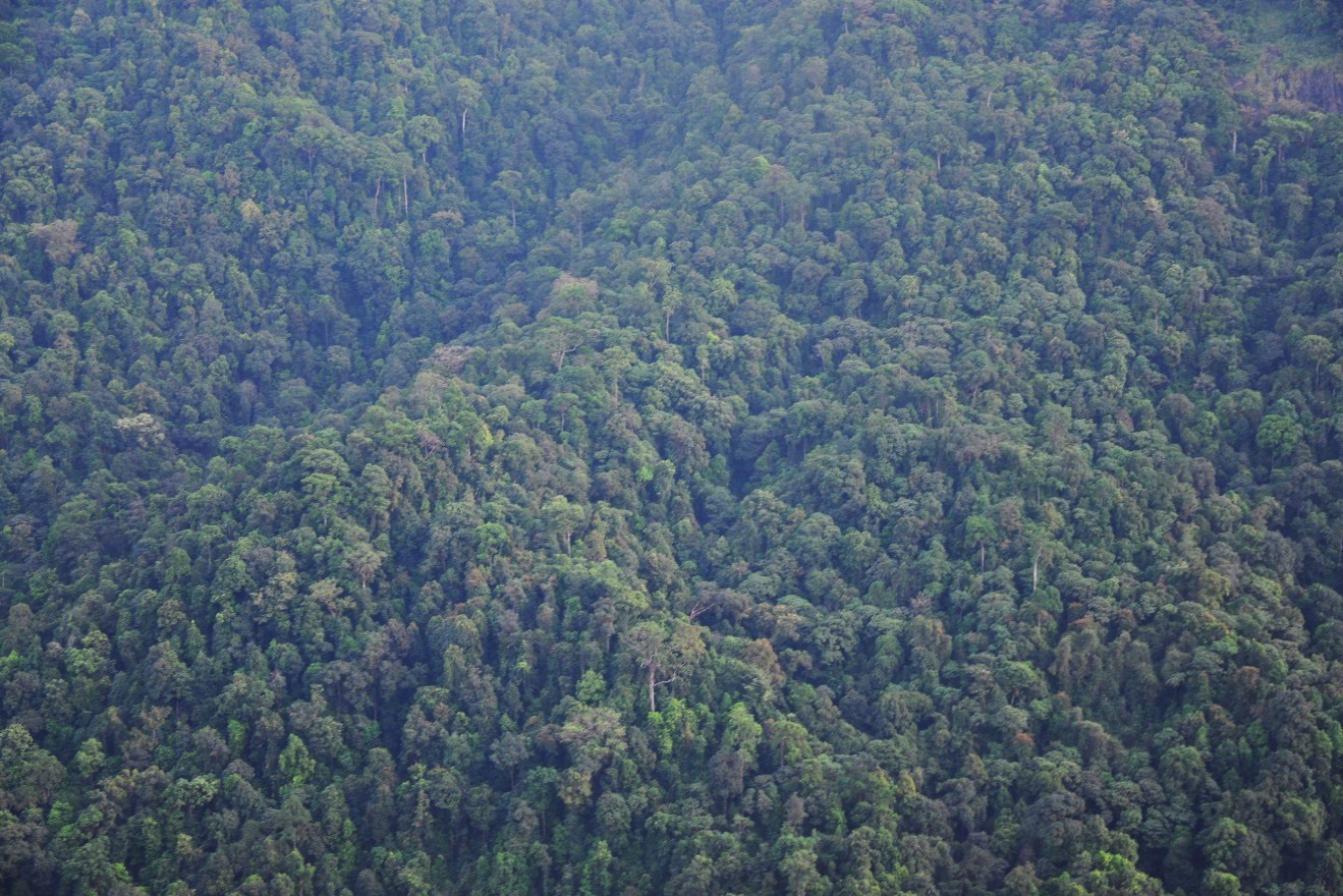
Figure 3.1.18: Pushpagiri Wild life Sanctaury
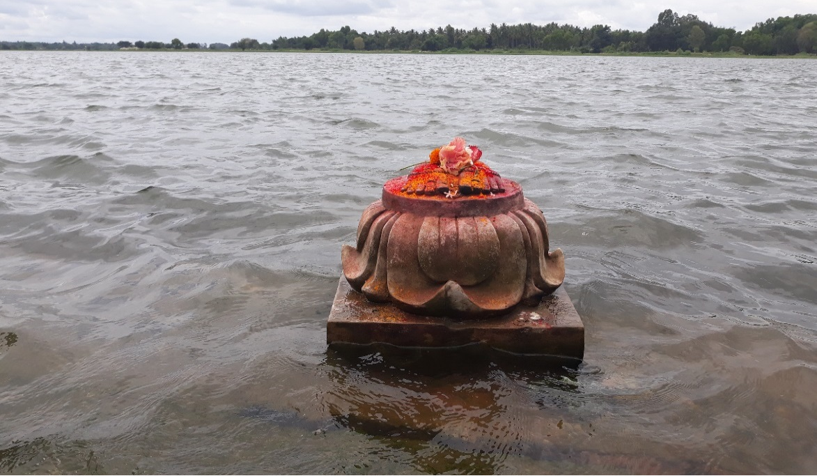

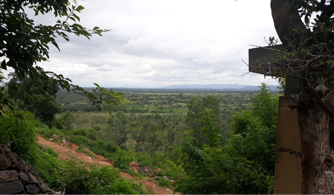

Figure 3.1.19 : Cauvery River and Landscapes near Talakadu

Figure 3.1.20: Agriculture land – Hassan
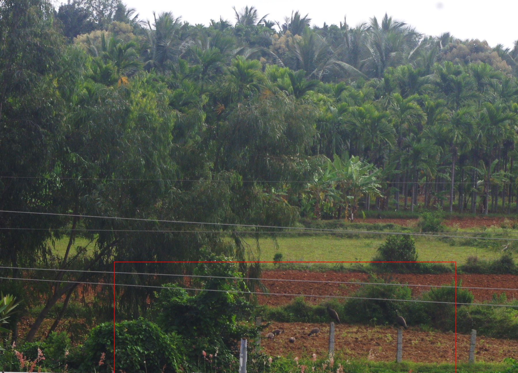
Figure 3.1.21 : Peafowls in agriculture field near Adichunchanagiri peacock sanctuary
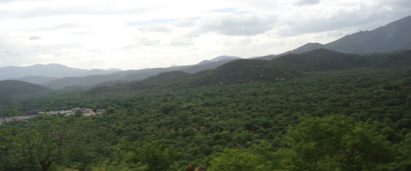
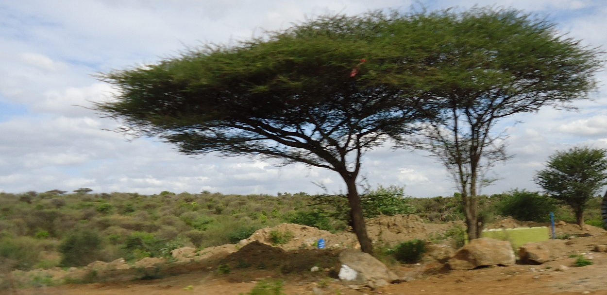
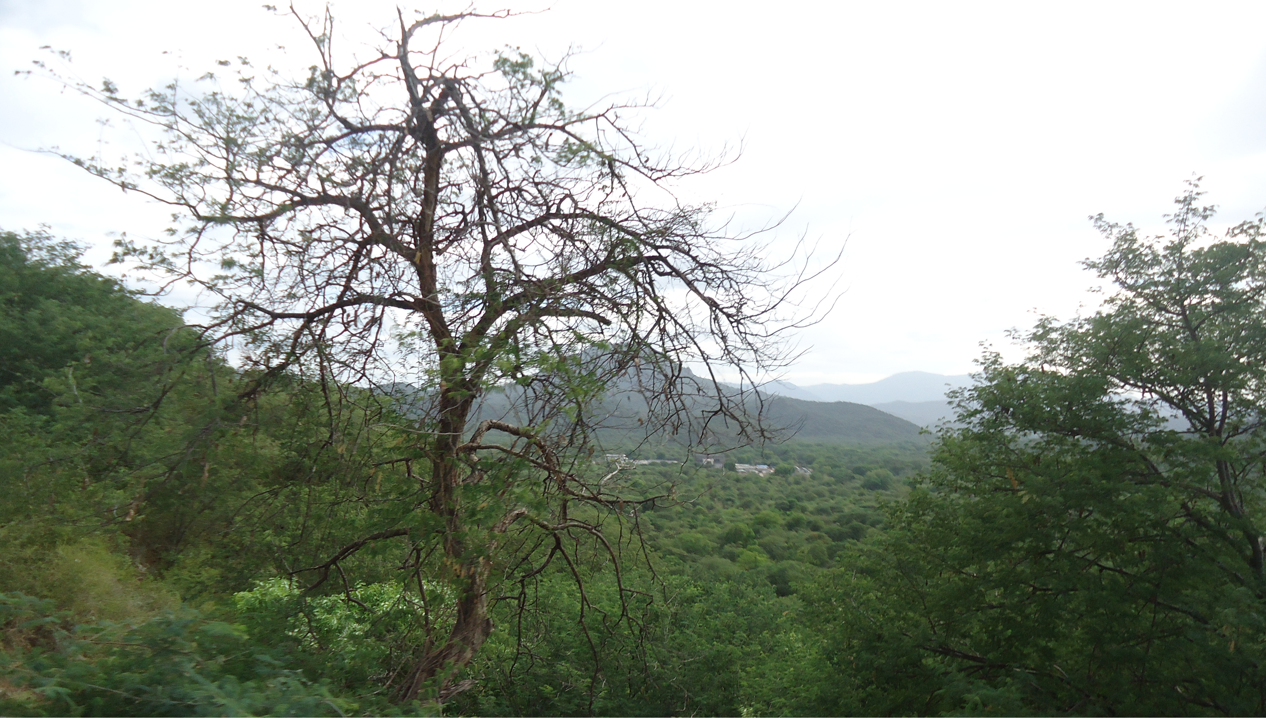
Figure 3.1.22 : Dry deciduous forest cover at Dharmapuri region (Near Hoginekal falls)

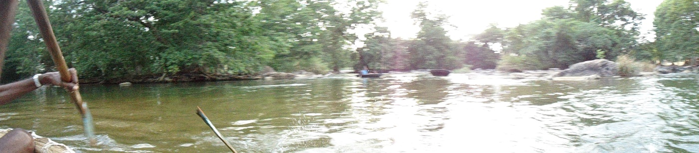
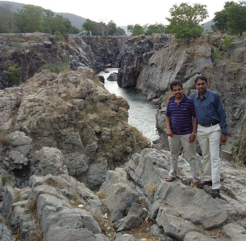

Figure 3.1.23 : Cauvery near Hoginekal

Figure 3.1.24: Dry deciduous forest of Satyamangalam Wild Life Sanctuary
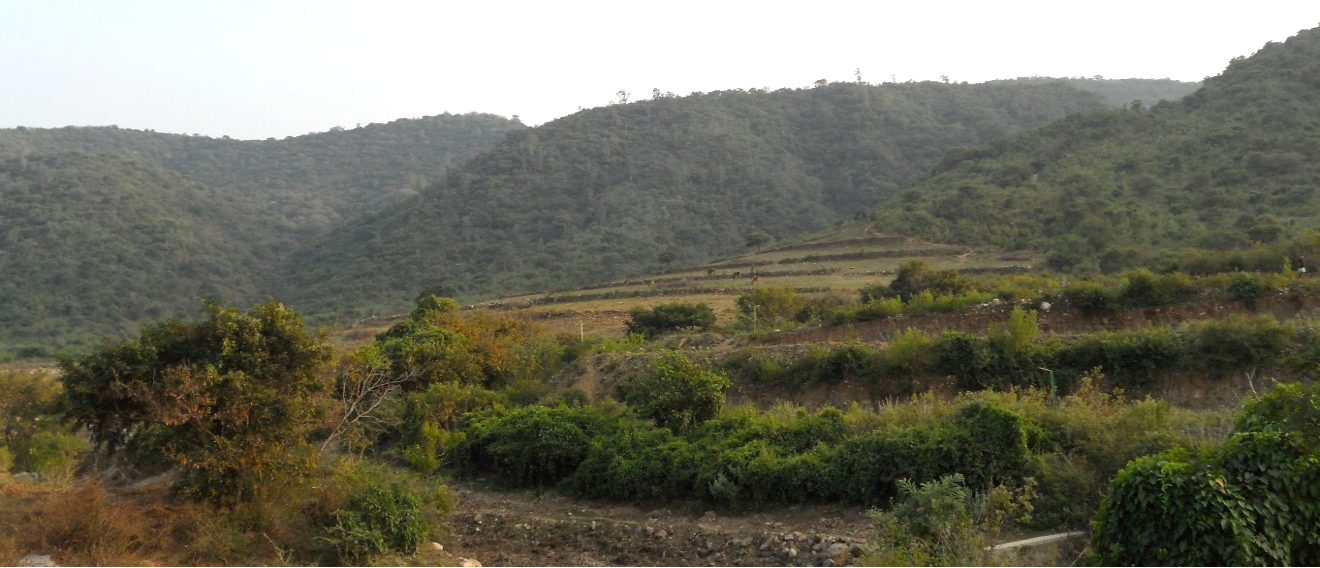
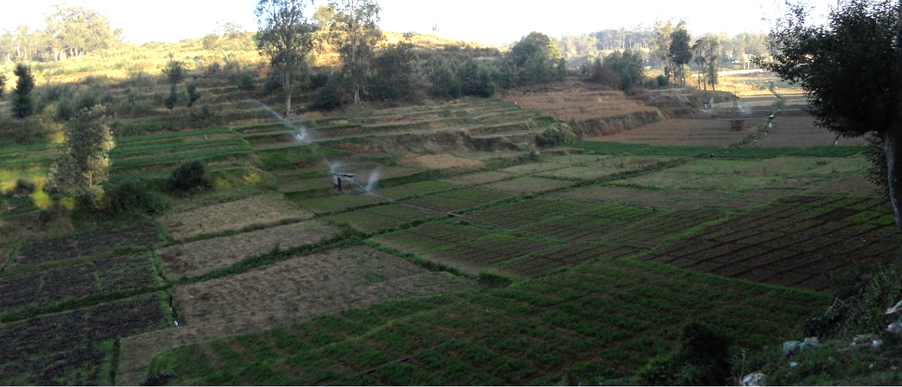
Figure 3.1.25: Attapadi hills (dry to mist deciduous) near Silent Valley National Park-step culture agriculture system

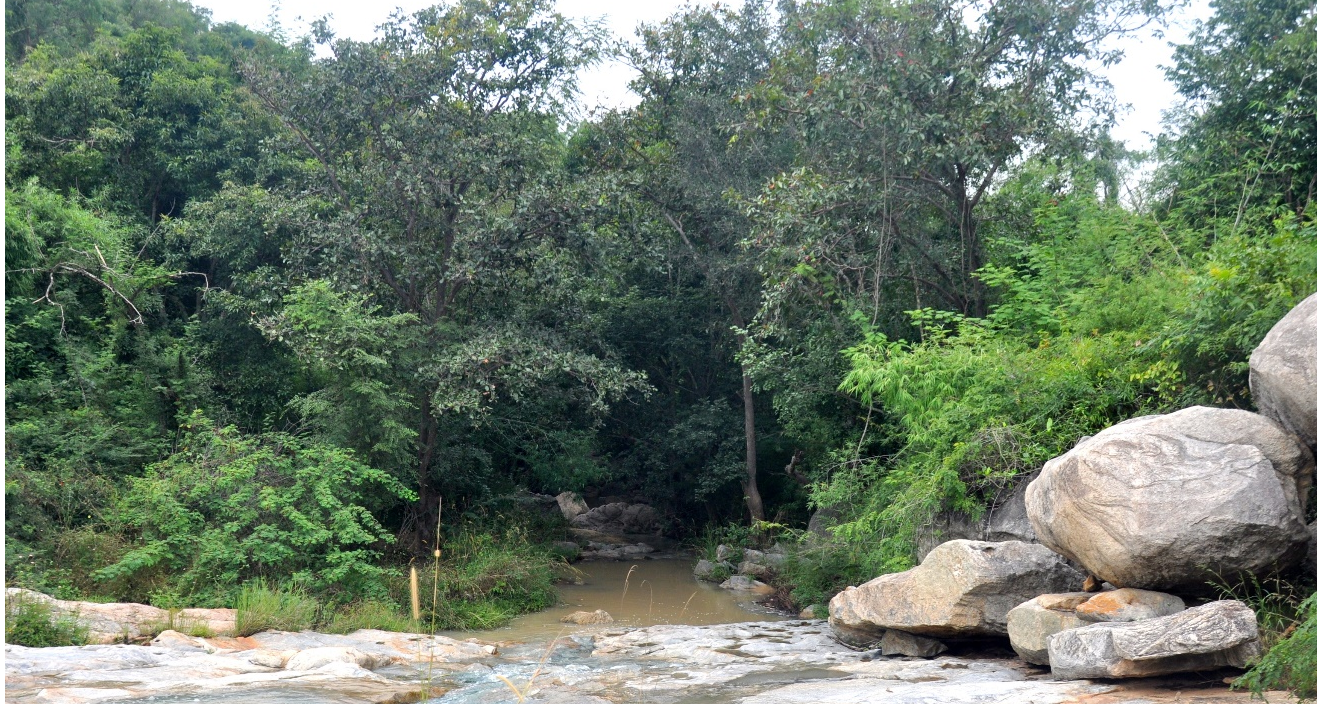
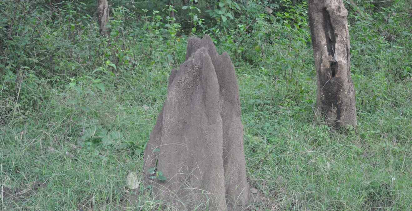
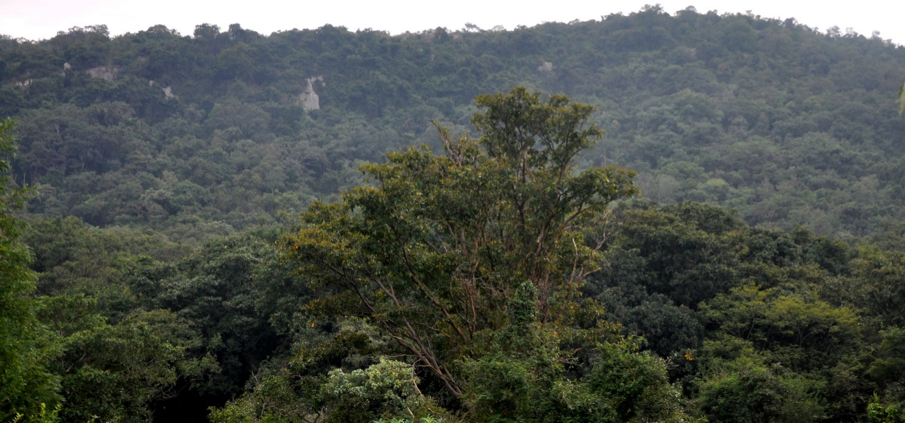

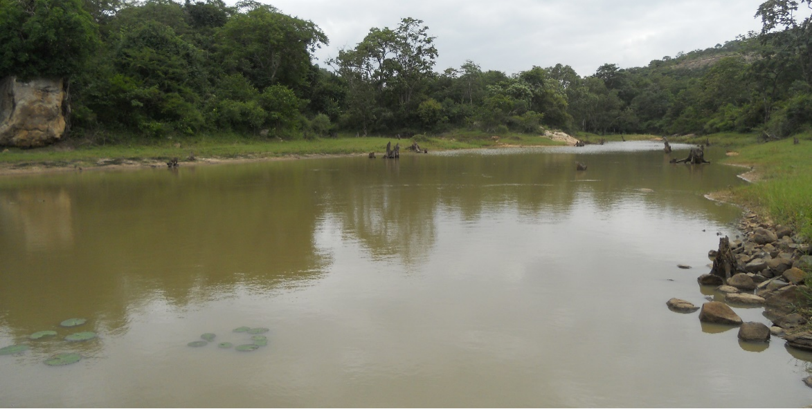


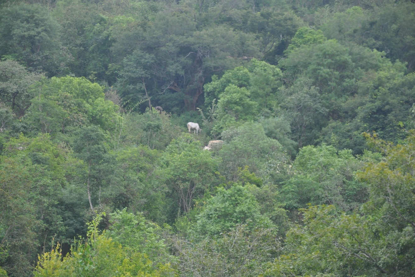


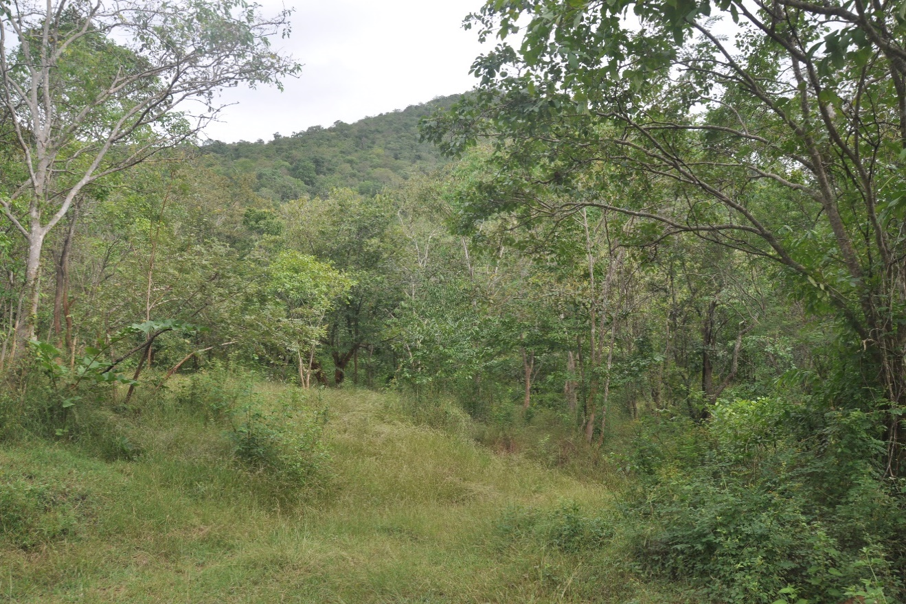
Figure 3.1.26: Bannerghata National Park – Land scapes

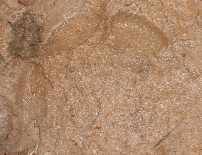


Figure 3.1.27: Wild life Sighthing and Signatures (Elephant, Tiger pug mark, Wild bison, Deer) Bannerghata National Park
Figure 3.1.28: Mulberry Cultivation in BNP and its surrounding villages
Figure 3.1.29: Agriculture field with bobbed wire to protect from wild animal (electrical connection provided during night).

Figure 3.1.30: Sand Mining – BNP

Figure 3.1.31: Gomala Land - BNP
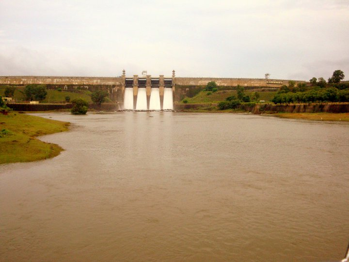
Figure 3.1.32: Harangi Dam
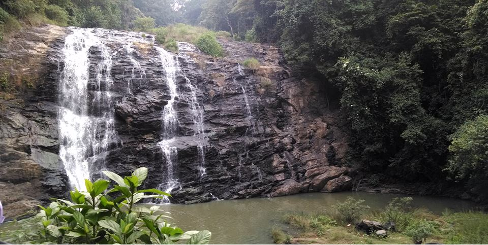
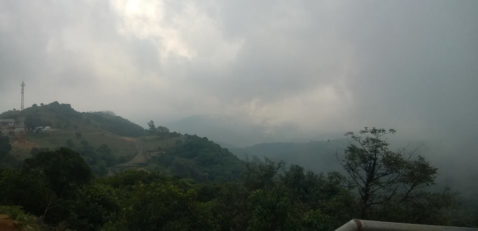


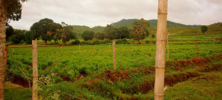

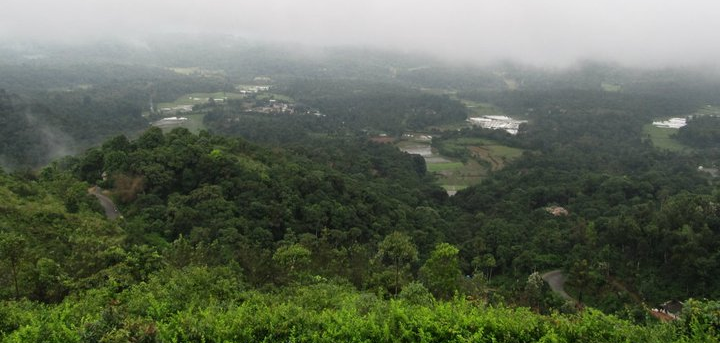
Figure 3.1.33: Landscapes – Madikeri
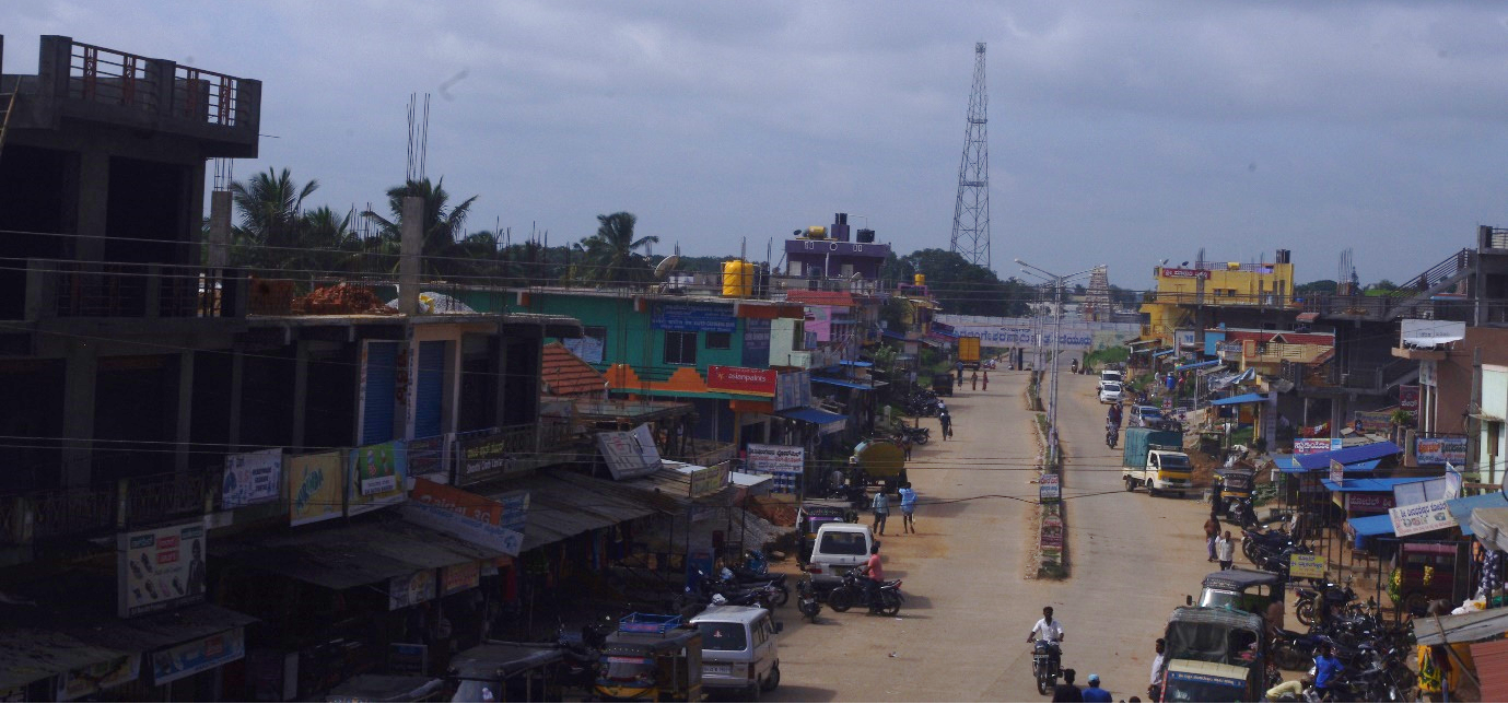

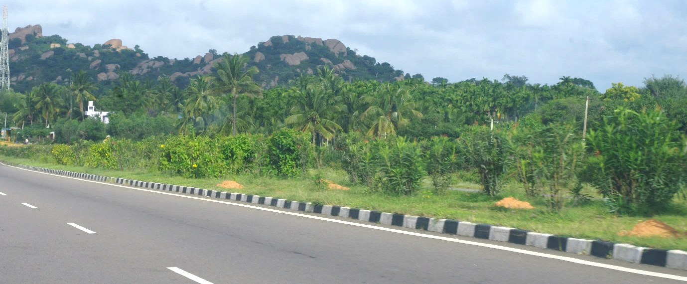
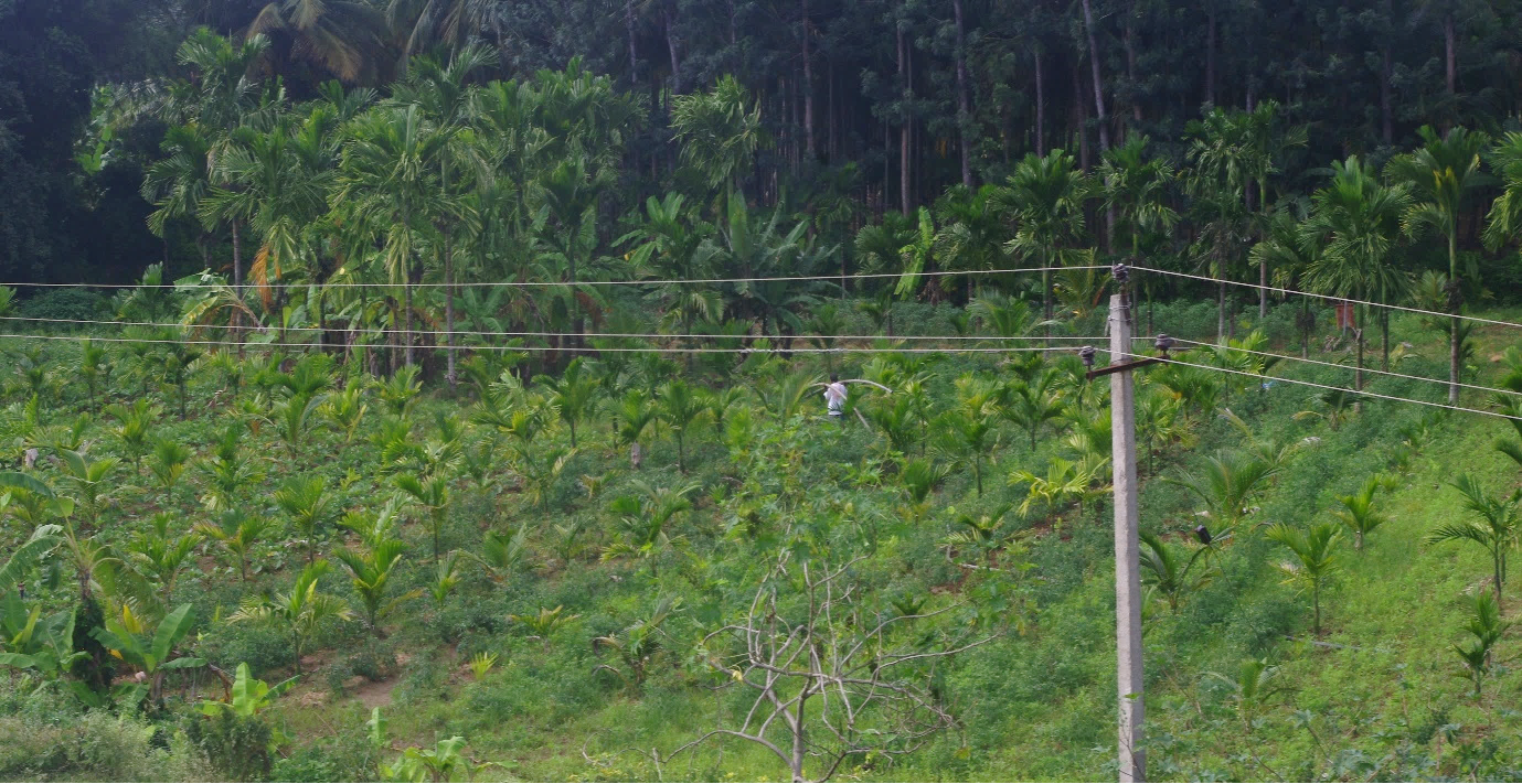
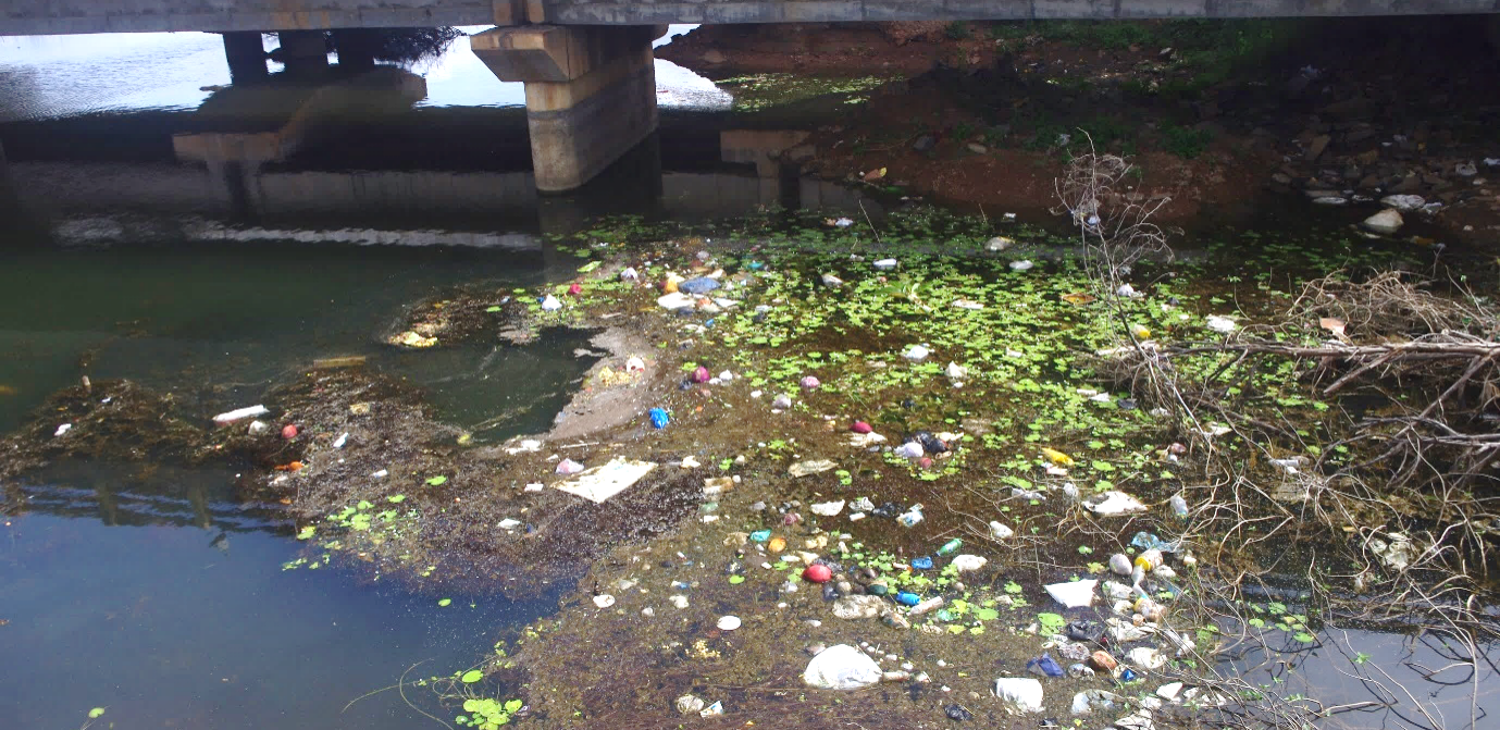
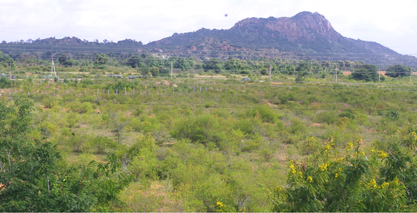


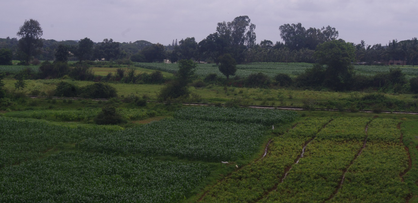

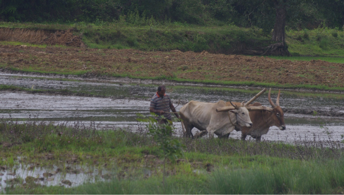

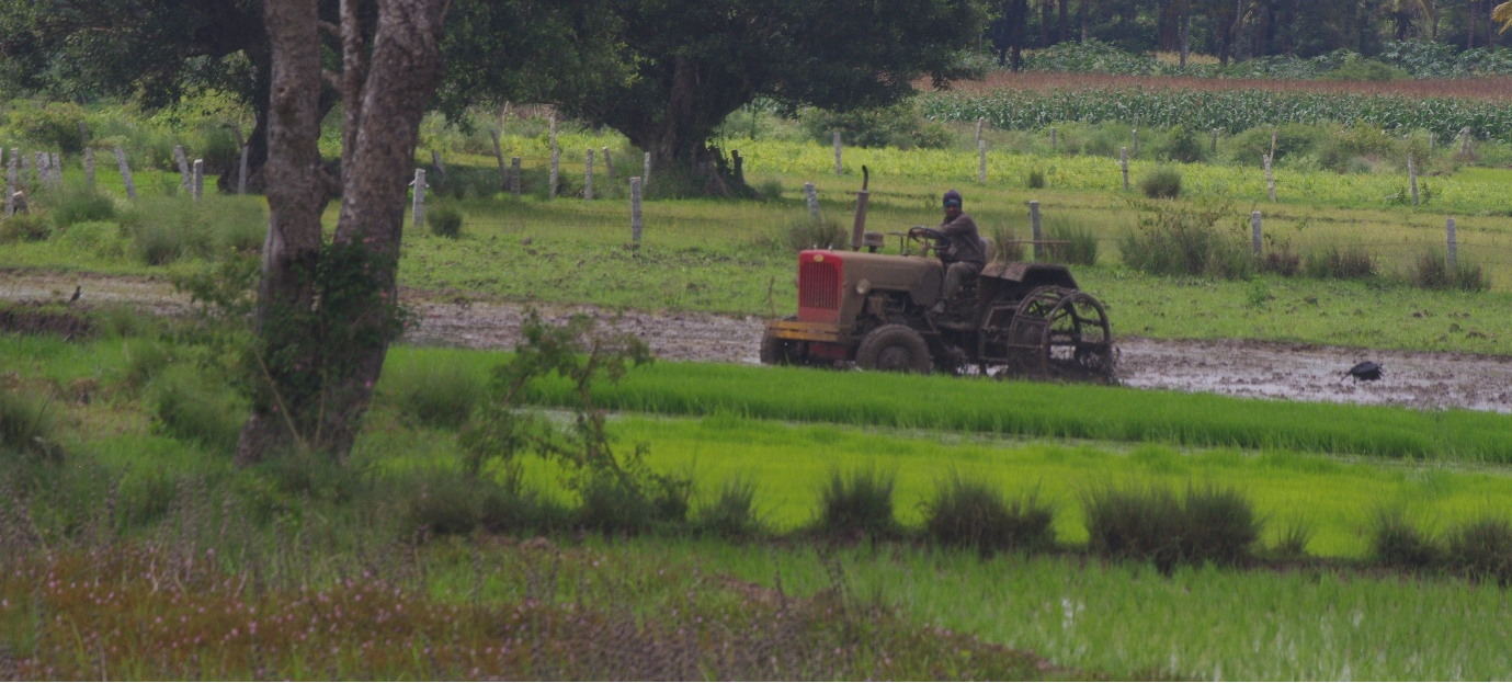
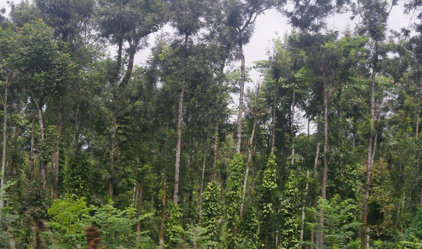
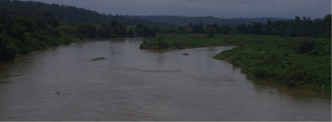
Figure 3.1.34: Landscapes – Bangalore to Sakleshpur

Figure 3.1.35: Mettur Dam [49]
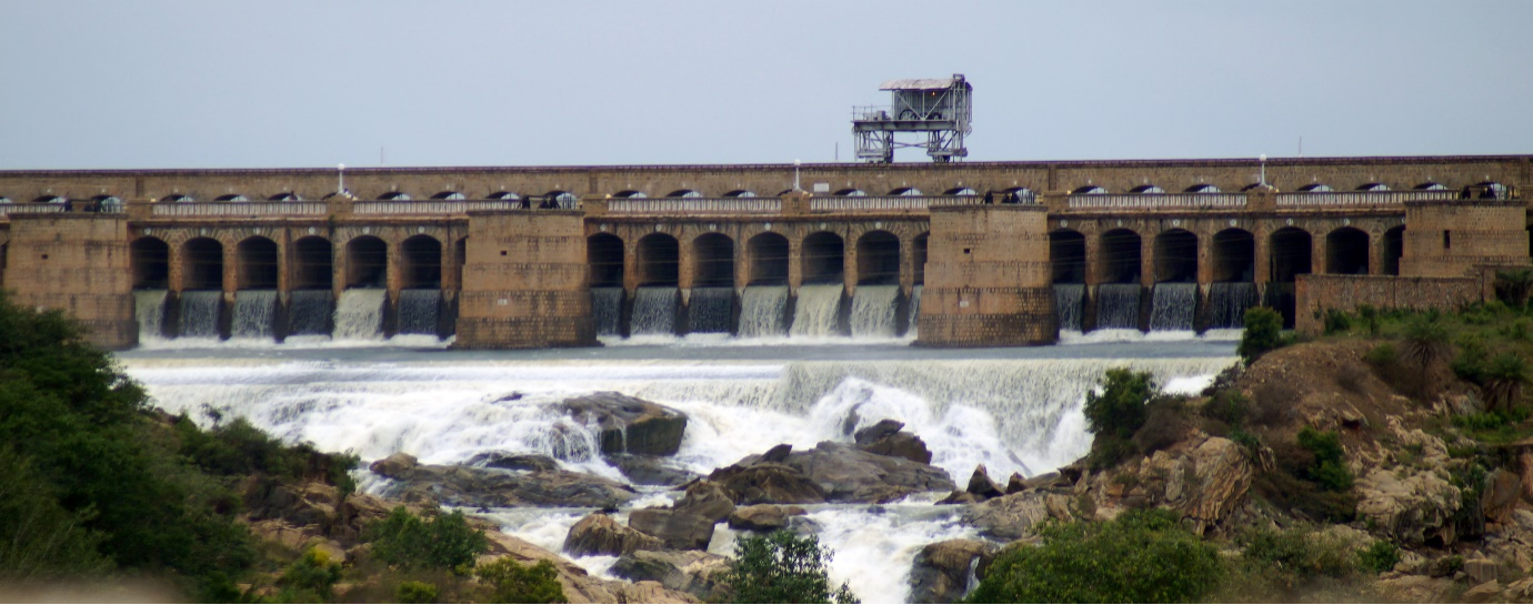
Figure 3.1.36: Krishna Raja Sagara Dam [2]
Figure 3.1.37: Talakaveri [2]

Figure 3.1.38: The Grand Anicut [2]

Figure 3.1.39 : Landscape Coimbatore
3.2. METHOD
3.2.1 LAND USE
Land use classification based on spatial pattern recognition technique applied on multi spectral remote sensing data is one of the common method used for image analysis to derive information [50]. The method adopted for land use classification is described in Figure 3.2.1.1. Process of land use classification is executed in three phases i) Data Acquisition, ii) Data Preprocessing and iii) Classification
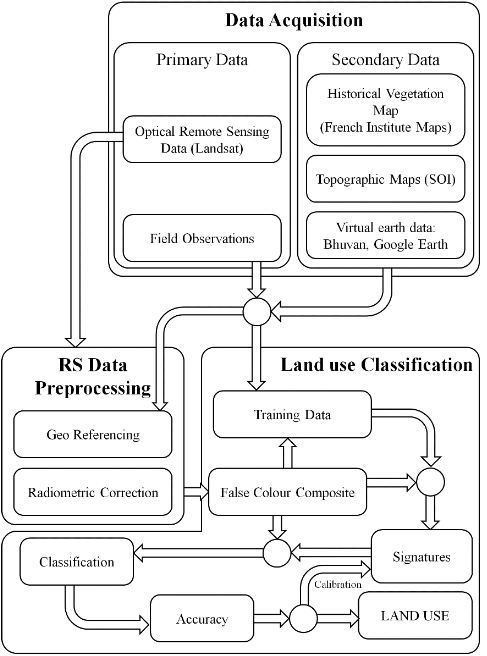
Figure 3.2.1.1: Method involved in understanding Land use
i) Data Acquisition: The process of data acquisition involves collection of Primary and Secondary Data. Primary Data includes collection of Remote Sensing Data and Field Data. Remote Sensing Data about 10 scenes of Landsat 8 for the year 2016 was downloaded from USGS web portal [17]. GPS and AGPS based field surveys were done in order to supplement land use analysis. Secondary Data collection involves collection of ancillary data such a French institute Puducherry vegetation maps [51], Geographical Survey of India topographic land use maps [52], Biodiversity portal[53]and Virtual earth data such as Google Earth [5], Bhuvan [54]. The Secondary data provides additional input to the field data for data pre-processing and classification.
ii) Data Preprocessing: Data Preprocessing involves Geo-referencing and Radiometric correction of RS data. GPS based field data along with Google earth, Bhuvan are to geo-reference the remote sensing data. Error up to 30 meter (1 pixel) was allowed during the process of Geo-referencing the data.RS data was checked for radiometric errors and enhancement was carried out for those datasets having errors. The correct image was cropped to the area of interest (Cauvery Basin).
iii) Classification: Image classification is a process of producing thematic map by assigning categories to each pixel based on the spectral signatures obtained from stack of multi band RS data [55]–[60]. The process of classification involves the following steps
- Creation of False Colour Composite which helps in identifying heterogeneous feature. NIR, Red and Green bands are stacked to create an FCC.
- Creating of Training Data Sites: Secondary data and Field data are used in association with Remote Sensing data to delineate heterogeneous features covering at least 15% of the scene area. Features such as Forests (evergreen, deciduous, scrub, mixed forest), Grass lands, Built-up, Agriculture (Sown and Fallow), Plantation (Coconut, Rubber, Tea, Coffee, etc.), Water bodies, Others (Quarry, Sand, Open lands, Rocky outcrops) were identified and Training data were delineated.
- Signatures: Optical bands of Landsat 8 (Blue, Green, Red, NIR, SWIR 1, SWIR2) were stacked. The Training datasets were overlaid on the RD data stack and signatures were prepared for each Feature Class. Of all the signatures, 60% were used for classification and 40% were used for Accuracy assessment.
- Classification: The signatures were used to classify the stacked RS data into various land use classes based on supervised pattern classification technique. Maximum likelihood classifier is one of the most commonly used classification tool[61]–[65] was used to classify the data into various land use classes.
- Accuracy Assessment: Accuracy assessment was carried out to understand how close the classified land use image to the reference map / ground data. 40% of the Signatures were used for measuring accuracy of the classified output. If the accuracy was below 80%, process was repeated by adding additional training data sites and classifying the data.
3.2.2 CONSERVATION RESERVE
The land use analysis of PAs is carried out to understand status of forest cover and their significance in conservation. Land use analyses involved (i) generation of False Color Composite (FCC) of remote sensing data (bands-green, red and NIR). This composite image helps in locating heterogeneous patches in the landscape, (ii) selection of training polygons by covering 15% of the study area (polygons are uniformly distributed over the entire study area) (iii) loading these training polygons co-ordinates into pre-calibrated GPS, (vi) collection of the corresponding attribute data (land use types) for these polygons from the field. GPS helped in locating respective training polygons in the field, (iv) supplementing this information with Google Earth and (v) 60% of the training data has been used for classification, while the balance is used for accuracy assessment. The land use analysis was done using supervised classification technique based on Gaussian maximum likelihood (GML) algorithm with training data (collected from field using GPS). GRASS GIS (Geographical Resources Analysis Support System) [66], [67], a free and open source software with the robust support for processing both vector and raster data has been used for analyzing RS data by using available multi-temporal “ground truth” information
3.2.3 BIODIVERSITY: FLORA FAUNA DISTRIBUTION
The current research work tries to understand and map the wealth of biodiversity in Cauvery basin by reviewing respective literatures and data collected from field visits. The details of faunal and floral species and their ecological significance, threat status are collected for comprehensive understanding of this rich biodiversity hotspot.
Field visit were undertaken in certain locations for flora composition through quadrat based study, 10 x 10 m quadrats were laid for accessing tree diversity, dominance and per hectare basal area. In each quadrat all trees > 30 cm were enumerated with their GBH (Girth at breast height) and height (m). In the same quadrat one 5 x 5 m shrub plot were laid and tree saplings and shrubs above 1 m were recorded. Two herb plots of 1 x 1 m were laid in each opposite ends to enumerate the seedlings. Opportunistic plant recording was also carried out in inaccessible areas. Along with vegetation data other details regarding plant-animal interaction, human-wildlife conflicts, etc., were noted. Literatures were reviewed and compiled a list of total number of floral species, faunal species including Fishes, Amphibians, Reptiles, Birds and Mammals present in the basin (Figure 3.2.3.1). Authenticity of the articles was ascertained before compiling the information. Location details including the geographical coordinates of species sightings were collected from the reviewed articles itself. Other relevant information such as conservation status, endemism, Legal protection, Habitat details and taxonomical details of each species were collected from IUCN Red List [68], India Biodiversity Portal [69] and ENVIS Sahyadri: Western Ghats Biodiversity Information System databases [70]. Querying was done with respect to the Species name, Family name, Conservation status and Endemism. Distribution maps for various categories included in the conservation status are prepared such as critically endangered, endangered, vulnerable, near threatened, least concern, data deficient and not evaluated.

Figure 3.2.3.1: Method followed for preparation of flora faunal maps.
3.2.4 RAINFALL DYNAMICS
Long term monthly precipitation data was collected from the open source database of Global Precipitation Climatology Centre, Earth System Research Observatory [71] of NOAA, United States. GPCC data downloaded has a spatial resolution of 0.25o X 0.25o between 1901 to 2013 in NetCDF format. The data was preprocessed (Geo referenced) and QGIS-LasPlamas [72] (version 2.18.12) was used to read the file. Gridded Point map were created to extract precipitation data from GPCC. Monthly precipitation data was extracted using Point Sampling Tool of QGIS. The data was further analyzed for assessing trend, frequency, dependability, return period, excess, drought cases and other conditions both State and Agro climatic zone wise [73]. Figure 3.2.4.1 depicts the method involved in understanding the temporal dynamics of precipitation.

Figure 3.2.4.1: Method involved in understanding temporal dynamics of precipitation data
India Meteorological Department [74] classifies rainfall at regional scale as Excess, Normal, Deficient/Drought, Scanty/Severe Drought conditions.
- Excess: Rainfall > + 20% average annual rainfall
- Normal: - 20% average annual rainfall < Rainfall < + 20% average annual rainfall
- Deficient: - 60% average annual rainfall < Rainfall < - 20% average annual rainfall
- Scanty: - 99% average annual rainfall < Rainfall < - 60% average annual rainfall
Further to understand the rainfall dynamics across seasons, and integration of data through GIS was done for hydrological analysis. Higher resolution monthly precipitation data of 1 km grid was downloaded from WorldClim-Global Climate Data [10], [11]. WorldClim data is an open source data consisting of average monthly climate data for minimum, mean, and maximum temperature (oC) and for precipitation (mm) for 1970-2000, in addition, Solar Radiation (kJ/m2/day), Wind speed (m/s), Water vapor pressure (kPa) and Bioclimatic variables at resolutions of 10’, 5’, 2.5’, 30” are available. The world level data from WorldClim was extracted to basin level for understanding seasonal variations in rainfall across the administrative boundaries.
3.2.5 HYDROLOGY AND COMPUTATION OF PARAMETERS
3.2.5.1 Runoff: Estimate runoff was based on the Natural Resource Conservation Series (NRCS) [75]–[78] earlier known as Soil Conservation Series (SCS) [79], [80] runoff curve number method. NRCS method (Figure 3.2.5.1) involves quantification of runoff considering precipitation data, land use, soil characteristics.
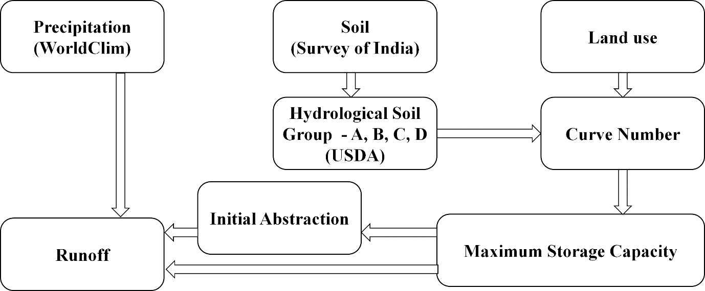
Figure 3.2.5.1: Steps involved in NRCS method of Runoff quantification
Mathematically Yield using NRCS is given as
Q= ((P-Ia )2 ) / ((P-Ia )+S)
Where
Q - Discharge/Yield as mm,
P - Precipitation in mm,
Ia - Initial Abstraction in mm,
S – Maximum Storage/Retention Potential in mm
Initial Abstraction (Ia) consists mainly interception, portion of infiltration and surface depression storage. In general, Ia is estimated based on landscape and surface conditions. Ia is estimated as function of maximum potential retentions (S). Ia is generalized as 20% of maximum storage capacity [77], whereas for Indian conditions, Ia can be taken as 30% of maximum potential storage [81]
Maximum retention potential is estimated as a function of curve number [82]and is given by
S=25.4*( ((1000)/(CN))-10)
CN represents curve number and is dependent on Soil Hydrological characteristics (Hydrological Soil Group) and Land use characteristics.
Hydrologic Soil group is defined by various soil properties such as density, texture, particle size, etc. which defines infiltration rates, storage capabilities of soil. Table 3.2.5.1 provides the details of HSG according national and international definitions and Table 3.2.5.2 provides the details of curve numbers associated with land use and soil group. The estimated runoff was validated with the field data.
Table 3.2.5.1: Hydrologic Soil Groups and their characteristics
|
HSG |
National [81], [83] |
International [84] |
|
A |
Sandy and Loamy Soils |
|
|
B |
Sandy Loamy and Loam |
|
|
C |
Clay loam |
|
|
D |
Clay |
|
Table 3.2.5.2: Curve numbers based on Land use and Hydrological Soil Group[85], [86]
|
Sl.no. |
Land use |
Hydrological condition |
A |
B |
C |
D |
|
1 |
Pasture, Grassland or range-continuous forage for grazing |
Poor |
68 |
79 |
86 |
89 |
|
Fair |
49 |
69 |
79 |
84 |
||
|
Good |
36 |
61 |
74 |
80 |
||
|
2 |
Meadow - continuous grass, protected from grazing and generally moved for hay |
Good |
30 |
58 |
74 |
78 |
|
3 |
Brush-weed -grass mixture with Brush as major element |
Poor |
48 |
67 |
77 |
83 |
|
Fair |
35 |
56 |
70 |
77 |
||
|
Good |
30 |
48 |
65 |
73 |
||
|
4 |
Woods- Grass combination (orchard or tree farm) |
Poor |
57 |
73 |
82 |
86 |
|
Fair |
43 |
65 |
76 |
82 |
||
|
Good |
32 |
58 |
72 |
79 |
||
|
5 |
Woods |
Poor |
45 |
66 |
77 |
83 |
|
Fair |
36 |
60 |
73 |
79 |
||
|
Good |
30 |
55 |
70 |
77 |
||
|
6 |
Farmstead - Buildings, lanes, drive ways and surrounds |
- |
59 |
74 |
82 |
86 |
|
7 |
Open space |
Poor |
68 |
79 |
86 |
89 |
|
Fair |
49 |
69 |
79 |
84 |
||
|
Good |
39 |
61 |
74 |
80 |
||
|
8 |
Impervious areas |
|||||
|
Paved parking lots, roofs and drive ways, etc. |
|
98 |
98 |
98 |
98 |
|
|
Streets and Roads |
||||||
|
Paved; curbs and storm sewers |
|
83 |
89 |
92 |
93 |
|
|
Paved; open ditches |
|
76 |
85 |
89 |
91 |
|
|
Gravel |
|
76 |
85 |
89 |
91 |
|
|
Dirt |
|
72 |
82 |
87 |
89 |
|
|
9 |
Urban Area |
|||||
|
Commercial |
85 % impervious |
89 |
92 |
94 |
95 |
|
|
Industrial |
72% impervious |
81 |
88 |
91 |
93 |
|
|
Residential |
65% impervious |
77 |
85 |
92 |
92 |
|
|
38% impervious |
61 |
75 |
83 |
87 |
||
|
30% impervious |
57 |
72 |
81 |
86 |
||
|
25% impervious |
54 |
70 |
81 |
85 |
||
|
20% impervious |
51 |
68 |
79 |
84 |
||
|
12% impervious |
46 |
65 |
77 |
82 |
||
|
10 |
Herbaceous : mixture of grass weed an low growing brush |
Poor |
|
80 |
87 |
93 |
|
Fair |
|
71 |
81 |
89 |
||
|
Good |
|
62 |
84 |
85 |
||
|
11 |
Oak-aspen : Mountain bush mixture of oak brush, aspen, mahogany, maple and other |
Poor |
|
66 |
74 |
79 |
|
Fair |
|
48 |
57 |
63 |
||
|
Good |
|
30 |
41 |
48 |
||
|
12 |
Pinyon-juniper: Pinyon, Juniper or both; grass understory |
Poor |
|
75 |
85 |
89 |
|
Fair |
|
58 |
73 |
80 |
||
|
Good |
|
41 |
61 |
71 |
||
|
13 |
Sage with grass understory |
Poor |
|
67 |
80 |
85 |
|
Fair |
|
51 |
63 |
70 |
||
|
Good |
|
35 |
47 |
55 |
||
|
14 |
Desert Shrub: saltbush, greasewood, cactus, mesquite, etc. |
Poor |
63 |
77 |
85 |
88 |
|
Fair |
55 |
72 |
81 |
86 |
||
|
Good |
49 |
68 |
79 |
84 |
||
|
Agriculture |
||||||
|
15 |
Fallow Land |
|||||
|
Bare Soil |
|
77 |
86 |
91 |
94 |
|
|
Crop Residue |
Poor |
76 |
85 |
90 |
93 |
|
|
Good |
74 |
83 |
88 |
90 |
||
|
16 |
Row Crops |
|||||
|
Straight Row |
Poor |
72 |
81 |
88 |
91 |
|
|
Good |
67 |
78 |
85 |
89 |
||
|
Crop Residue + Straight Row |
Poor |
71 |
80 |
87 |
90 |
|
|
Good |
64 |
75 |
82 |
85 |
||
|
Contoured |
Poor |
70 |
79 |
84 |
88 |
|
|
Good |
65 |
75 |
82 |
86 |
||
|
Contoured + Crop Residue |
Poor |
69 |
78 |
83 |
87 |
|
|
Good |
64 |
74 |
81 |
85 |
||
|
Contoured + Terraced |
Poor |
66 |
74 |
80 |
82 |
|
|
Good |
62 |
71 |
78 |
81 |
||
|
Contoured + Terraced + Crop residue |
Poor |
65 |
73 |
79 |
81 |
|
|
Good |
61 |
70 |
77 |
80 |
||
|
17 |
Small Grains |
|||||
|
Straight Row |
Poor |
65 |
76 |
84 |
88 |
|
|
Good |
63 |
75 |
83 |
87 |
||
|
Crop Residue + Straight Row |
Poor |
64 |
75 |
83 |
86 |
|
|
Good |
60 |
72 |
80 |
84 |
||
|
Contoured |
Poor |
63 |
74 |
82 |
85 |
|
|
Good |
61 |
73 |
81 |
84 |
||
|
Contoured + Crop Residue |
Poor |
62 |
73 |
81 |
84 |
|
|
Good |
60 |
72 |
80 |
83 |
||
|
Contoured + Terraced |
Poor |
61 |
72 |
79 |
82 |
|
|
Good |
59 |
70 |
78 |
81 |
||
|
Contoured + Terraced + Crop residue |
Poor |
60 |
71 |
78 |
81 |
|
|
Good |
58 |
69 |
77 |
80 |
||
|
18 |
Close Seeded or Broadcast Legumes or Rotation Meadows |
|||||
|
Straight Row |
Poor |
66 |
77 |
85 |
89 |
|
|
Good |
58 |
72 |
81 |
85 |
||
|
Contoured |
Poor |
64 |
75 |
83 |
85 |
|
|
Good |
55 |
69 |
78 |
83 |
||
|
Contoured + Terraced |
Poor |
63 |
73 |
80 |
83 |
|
|
Good |
51 |
67 |
76 |
80 |
||
3.2.5.2 Infiltration: Infiltration is the amount of water that enters through soil surface replenishing soil moisture and building up ground water table [86]. Infiltration is estimated as function of rainfall, catchment conditions, runoff, interception and evapotranspiration (Figure 3.2.5.2). Interception is quantified across different vegetative landscape based on interception equations as shown in table 3.2.5.3.
Infiltration = Precipitation – (Runoff + Interception + Evapotranspiration)
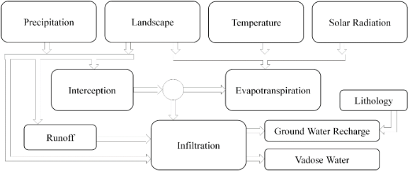
Figure 3.2.5.2: Method involve in estimating Infiltration
Table 3.2.5.3: Interception equations [87]
|
Vegetation types |
Interception |
|
Evergreen/semi-evergreen forests |
I = 5.5 + 0.3 (P) |
|
Moist deciduous forests |
I = 5 + 0.3 (P) |
|
Plantations |
I = 5 + 0.2 (P) |
|
Grasslands and scrubs |
I = 3.5 +0.18 (P) |
3.2.5.3 Ground Water Recharge: Ground Water recharge was estimated as function of Porosity of sub strata and Annual Average Rainfall. Porosity of various rock types [86], [88], [89] are as presented in Table 3.2.5.4.
Table 3.2.5.4: Porosity of Rocks
|
Rock Type |
Porosity |
|
Alluvial area Sandy |
20 - 25% |
|
Alluvial area Clayey |
10 - 20% |
|
Limestone Sandstone, Phyllite, Shale |
10 - 20% |
|
Basaltic - Vesicular |
10 - 15% |
|
Basaltic- Weathered |
4 - 10% |
|
Granite Weathered |
10 -15% |
|
Granite Unweather |
5 - 10% |
3.2.5.4 Evapotranspiration: Potential evapotranspiration (PET) is determined using Hargreaves method [90–93] which is a radiation based equation (Figure 3.2.5.3). PET is estimated as mm using the Hargreaves equation is given as
PET=0.0023* ((RA)/λ) * √(T(max) -T(min) ) *( (T(max) +T(min) )/2+17.8)
Where RA is Extra-terrestrial radiation (MJ/m2/day) which depends on the latitudinal gradients[94], Tmax is Maximum temperature in degree Celsius [11], Tmin Minimum Temperature in degree Celsius [11] and λ is latent heat of vaporization of water (2.501 MJ/kg)[95]. Actual evapotranspiration is estimated as a product of Potential evapotranspiration (PET) and Evapotranspiration coefficient (KC)[96].
Table 3.2.5.5: Evapotranspiration coefficients
|
Land use |
KC |
|
Built-up |
0.15 |
|
Water |
1.05 |
|
Open space |
0.3 |
|
Semi-evergreen moist deciduous forest |
0.95 |
|
Evergreen forest |
0.95 |
|
Scrub and grassland |
0.8 |
|
Acacia |
0.85 |
|
Teak and bamboo |
0.85 |
|
Dry-deciduous |
0.85 |
Note: Evapotranspiration was quantified only for nonagricultural landscape only. transpiration from agriculture and horticulture were quantified as a part of crop water demand
3.2.6 DOMESTIC, LIVESTOCK AND IRRIGATION WATER REQUIREMENTS
3.2.6.1 Domestic Water Demand: Domestic water demand is the amount of water required for the population in the catchment. Figure 3.2.6.1 depict the method involved in estimating domestic water requirement across sub basin level in the catchment.

Figure 3.2.6.1: Method involved in estimating Domestic Demand
Population data for each district in the basin was collected from census of India [7], based on the growth rate between 2001 and 2011, population for the year 2021 was predicted across the basin using simple interest method. Demand of 150 lpcd was considered to estimate domestic water demand in the basin. Proportional population was considered for districts which extends beyond the basin boundary.
Population 2021 = Population 2011 (1 + n.r)
Where r is the growth rate between 2011 and 2001, n is number of decades (= 1).
r= (Population 2011)/(Population 2001)-1
3.2.6.2 Livestock Demand: Similar to domestic demand, livestock demand was estimated considering livestock census across each districts [97]–[99]. Water demand for livestock was established through telephonic interviews and through literature[100], [101]. Table 3.2.6.1 provides insights to water demand for various livestock.
Table 3.2.6.1: Livestock Water demand
|
Livestock |
Cattle |
Buffalo |
Sheep |
Goat |
Pig |
Rabbit |
Dog |
Poultry |
|
Water ltr/animal |
70 -120 |
75 - 130 |
15 - 20 |
15 - 22 |
20 -30 |
1 - 2 |
6 – 10 |
0.25 – 0.35 |
3.2.6.3 Agricultural Demand: Agriculture demand depends on such as type of plant, growth phase of plant. In order to estimate crop water requirements, area under different at district level was established based on the statistical data published by the Government agencies [102]–[106]. Water requirement for each crop based on their growth phases[105], [107]–[111] were accounted to quantify agriculture demand.
3.2.7 HYDROLOGICAL STATUS: Hydrological status is estimated as a function of Demand and Available (water supply). It is a non-dimensional value indicating deficit or excess water availability in the region. Values greater than 1 indicate excess water, values equal to 1 indicate water availability and demands are equal, values less than 1 indicate deficiency.
Hydrological Status= (f(Water Supply))/(f(Water Demand)) = (f(Rainfall, Runoff, Infiltration, Evapotranspiration))/(f(Agriculture , Domestic and Livestock Demand))
3.2.8 SCENARIO BASED MODELING: Four scenarios were designed in order to address Hydrological status based on rainfall conditions and cropping pattern. Figure 3.2.8.1 and Table 3.2.8.1 describes the scenarios that have been used for the analysis. Since Paddy and Sugarcane are water intensive, reducing their cropping areas and growing less water intensive crops were considered for developing various scenarios. Scenario 1 and Scenario 2 were based on normal rainfall events, Scenario 3 and Scenario 4 were based on rainfall drought events.

Figure 3.2.8.1: Scenario development
Table 3.2.8.1: Scenario description with sustainable cropping pattern
|
Scenario |
Description of Each Scenario |
|
Normal rainfall Condition |
|
|
Scenario 1 |
|
|
Scenario 2 |
|
|
Rainfall drought Conditions |
|
|
Scenario 3 |
|
|
Scenario 4 |
|
Rainfall drought is estimated as function of Coefficient of Variation (COV) and average rainfall. Mathematically COV is defined as the ratio of standard deviation to the mean indicating the extent of variability in relation to mean. COV tries to explain the consistency of data, lower COV indicates higher dependability and vise-versa [112], [113] . COV was calculated across each Grid Point obtained from 113 year data obtained from GPCC[71], interpolation was carried out to understand the spatial variability of COV across the catchment. Rainfall drought was estimated as
Rainfall Drought = Actual Rainfall * (1 – COV)
Estimated Drought rainfall across seasons were used to quantify Runoff and other hydrological parameters, and incorporated in Scenarios 3 and 4.
Results & Discussion
4.1. LAND USE
Land use analysis was carried out for entire Cauvery river basin for the year 2016 (Landsat 8 OLI [1]) as shown in Figure 4.1.1 and Table 4.1.1. The analysis showed that the catchment was dominated by Agriculture activities (Agriculture and horticulture) i.e., about 73.5% followed by Forest cover which is about 18%. Dense forest area was 13.3% and Degraded forest area was nearly 4.63%.

Figure 4.1.1: Land use analysis of Cauvery River Basin.
Table 4.1.1: Land use in Cauvery river basin
|
Land use |
Area |
|
|
Sq.km |
% |
|
|
Dense Vegetation |
11,387.76 |
13.33 |
|
Degraded Vegetation |
3,957.91 |
4.63 |
|
Water |
1,210.74 |
1.42 |
|
Agriculture |
41,489.89 |
48.58 |
|
Plantation |
21,339.35 |
24.99 |
|
Built up |
3,112.89 |
3.65 |
|
Others |
2,907.95 |
3.41 |
|
TOTAL |
85,406.49 |
|
Comparing the forest cover dynamics across time, International Vegetation Maps developed by French institute Puducherry [2] was used as reference. Maps of Mysore, Madras and Cape Comorin of 1: 5,000,000 scale were used to extract natural cover in Cauvery river basin for the year 1965 - 1966. Natural vegetation cover during1965 (Figure 4.1.2) was nearly 33% (28194 sq.km) of which dense vegetation was about 20.5% (17510 sq.km) and degraded vegetation were about 12.5% (10684 sq.km). During this era, in the basin Karnataka portion had highest proportion of natural vegetation of 17073 sq.km (60.55%) cover followed by Tamil Nadu with 10078 sq.km (35.75%) and Kerala with 1044 sq.km (3.7%). Table 4.1.2 provides the details of natural vegetation cover across administrative boundaries within Cauvery Basin. Similarly based on the land use analysis for the year 2016 [1], Natural vegetation cover (Figure 4.1.3) was about 18 % (15345 sq.km) of which Karnataka portion had highest proportion of natural vegetation cover of 48.3% (7408 sq.km) followed by Tamil Nadu with 46.7% (7172 sq.km) and Kerala with 5% (764 sq.km). Table 4.1.3 provides detailed information on natural vegetation cover in the year 2016.
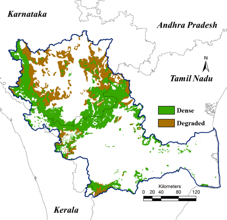
Figure 4.1.2: Natural Vegetation cover during 1965
Table 4.1.2: Vegetation Cover in Cauvery
River Basin in 1965.
|
Description |
Units |
Kerala |
Karnataka |
TN |
Puducherry |
Total |
|
|
Catchment Area |
sq.km |
2880.83 |
34936.80 |
47391.17 |
154.20 |
85363 |
|
|
Natural Vegetation Cover |
1965 Dense |
sq.km |
965.87 |
8667.82 |
7876.11 |
|
17510 |
|
% Veg |
5.5% |
49.5% |
45.0% |
|
|
||
|
% Geo |
33.5% |
24.8% |
16.6% |
|
20.5% |
||
|
1965 Degraded |
sq.km |
77.77 |
8404.99 |
2201.67 |
|
10684 |
|
|
% Veg |
0.7% |
78.7% |
20.6% |
|
|
||
|
% Geo |
2.7% |
24.1% |
4.6% |
|
12.5% |
||
|
1965 Total |
sq.km |
1044 |
17073 |
10078 |
|
28194 |
|
|
% Veg |
3.7% |
60.6% |
35.7% |
|
|
||
|
% Geo |
36.2% |
48.9% |
21.3% |
|
33.0% |
||
Note: TN: Tamil Nadu, % Veg - Percent of total vegetation cover and % Adm – Percent vegetation under each administrative division, within the catchment.

Figure 4.1.3: Natural Vegetation Cover in 2016
Table 4.1.3: Vegetation Cover in Cauvery River Basin in 2016
|
Description |
Units |
Kerala |
Karnataka |
Tamil Nadu |
Puducherry |
Total |
|
|
Catchment Area |
sq.km |
2880.83 |
34936.80 |
47391.17 |
154.20 |
85363 |
|
|
Natural Vegetation Cover |
2016 Dense |
sq.km |
707.74 |
5062.72 |
5616.71 |
|
11387 |
|
% Veg |
6.2% |
44.5% |
49.3% |
|
|
||
|
% Geo |
33.5% |
24.8% |
16.6% |
|
12.5% |
||
|
2016 Degraded |
sq.km |
56.41 |
2345.78 |
1555.72 |
|
3958 |
|
|
% Veg |
1.4% |
59.3% |
39.3% |
|
|
||
|
% Geo |
2.7% |
24.1% |
4.6% |
|
4.6% |
||
|
2016 Total |
sq.km |
764.16 |
7408.50 |
7172.42 |
|
15345.08 |
|
|
% Veg |
5.0% |
48.3% |
46.7% |
|
|
||
|
% Geo |
36.2% |
48.9% |
21.3% |
|
17.2% |
||
Note: % Veg - Percent of total vegetation cover and % Geo – Percent vegetation under each administrative division, within the catchment.
Between 1965 [2]and 2016[1], natural vegetation cover has reduced from 28194 sq.km to 15345 sq.km indicating that about 45.55% cover lost in 5 decades. dense vegetation has reduced by 35% (6123 sq.km) and degraded vegetation has reduced by 63% (6727 sq.km). Across the administrative divisions, Karnataka has lost about 57 % (9664 sq.km) followed by Tamil Nadu loosing 29% (2905 sq.km) and Kerala loosing 27% (279 sq.km) of the natural vegetation cover. Figure 4.1.4 and Table 4.1.4 describes the proportion of vegetation lost between 1965 and 2016.

Figure 4.1.4: Dynamics in natural vegetation cover
Table 4.1.4: Reduction in natural vegetation cover
|
Description |
Units |
Kerala |
Karnataka |
Tamil Nadu |
Total |
|
|
Dense Vegetation |
1965 |
sq.km |
965.87 |
8667.82 |
7876.11 |
17509.80 |
|
2016 |
sq.km |
707.74 |
5062.72 |
5616.71 |
11387.17 |
|
|
Loss |
sq.km |
258.12 |
3605.10 |
2259.40 |
6122.63 |
|
|
% |
27 |
42 |
29 |
35 |
||
|
Degraded Vegetation |
1965 |
sq.km |
77.77 |
8404.99 |
2201.67 |
10684.43 |
|
2016 |
sq.km |
56.41 |
2345.78 |
1555.72 |
3957.91 |
|
|
Loss |
sq.km |
21.36 |
6059.21 |
645.95 |
6726.52 |
|
|
% |
27 |
72 |
29 |
63 |
||
|
Total Natural Vegetation |
1965 |
sq.km |
1043.64 |
17072.81 |
10077.78 |
28194.23 |
|
2016 |
sq.km |
764.16 |
7408.50 |
7172.42 |
15345.08 |
|
|
Loss |
sq.km |
279.48 |
9664.31 |
2905.36 |
12849.15 |
|
|
% |
27 |
57 |
29 |
46 |
||
District wise forest dynamics is presented in Figure 4.1.5 and Table 4.1.5. Karnataka has highest forest cover of which Chamrajnagar District had the highest forest cover about 3300 sq.km followed by Mysore, Ramanagara, Kodagu and Hassan with forest cover over 2500 sq.km, Tamil Nadu has second largest forest cover with Erode having about 2300 sq.km, followed by Krishnagiri, The Nilgiris, Dharmapuri, Dindugal with over 1000 sq.km forest cover in 1965-1966. Forest cover has reduced across the basin, Tamil Nadu has higher forest degradation, districts such as Ariyur, Thanjavur, Pudukottai, Nagapattinam, Thiruvarur has lost over 90% forest cover in 5 decades and similar trend in parts of Karnataka, Districts such as Hassan, Mandya and Tumkur have lost over 70% forest cover in the catchment. Districts such as Chamarajnagar, Salem, Dindugal, Namakal, Tiruppur, Nilgiris, Krishangiri, Wayanad, Idukki, Palakkad, and Erode have forest degradation less than 40 %, other districts between 40 – 70% loss.
In Tamil Nadu, Erode among other districts, has the lowest forest loss i.e., about 22% (2351sq.km in 1966 – 1832 sq.km in 2016), similarly, in Karnataka, Chamrajnagara has lowest forest loss of 36% (3385 sq.km in 1965 – 2157 sq.km in 2016), Kerala, Palakkad and Waynad have 25 and 28% loss in forest cover.

Figure 4.1.5: Forest dynamics across District (Cauvery basin only)
Table 4.1.5: Forest Dynamics, District wise forest dynamics (Area in sq.km)
|
District |
1966 |
2016 |
% Forest Decline |
District |
1966 |
2016 |
% Forest Decline |
|
Chamrajnagar |
3385 |
2157 |
36% |
Bangalore |
545 |
194 |
64% |
|
Mysore |
2932 |
1064 |
64% |
Chikmagalur |
493 |
231 |
53% |
|
Ramanagara |
2564 |
1218 |
52% |
Tiruchirappalli |
381 |
178 |
53% |
|
Kodagu |
2554 |
1339 |
48% |
Namakkal |
379 |
244 |
35% |
|
Hassan |
2503 |
661 |
74% |
Palakkad |
367 |
274 |
25% |
|
Erode |
2351 |
1832 |
22% |
Tiruppur |
322 |
212 |
34% |
|
Krishnagiri |
1553 |
1105 |
29% |
Bangalore Rural |
123 |
47 |
62% |
|
The Nilgiris |
1381 |
915 |
34% |
Ariyalur |
115 |
6.5 |
94% |
|
Dharmapuri |
1278 |
742 |
42% |
Idukki |
96 |
71.3 |
26% |
|
Dindigul |
1158 |
746 |
36% |
Perambalur |
89 |
27.0 |
69% |
|
Mandya |
1057 |
274 |
74% |
Karur |
76 |
35.8 |
53% |
|
Tumkur |
917 |
224 |
76% |
Thiruvarur |
53 |
4.7 |
91% |
|
Salem |
712 |
437 |
39% |
Thanjavur |
29 |
1.4 |
95% |
|
Wayanad |
578 |
417 |
28% |
Pudukkottai |
17 |
0.8 |
95% |
|
Coimbatore |
565 |
438 |
23% |
Nagappattinam |
7 |
0.5 |
94% |
4.2. CONSERVATION RESERVE
The PAs are supporting flora and fauna species of diverse kind many are endemic to the specific region as shown in Figures 4.2.1 – 4.2.3. Forest cover and PAs of region are shown in Figure 4.2.4 signifies forested habitats with dense vegetation cover for effective conservation of forest dependent and endemic fauna, if forest cover in PAs is disturbed, then it will impact ecology of the whole basin.
 Figure 4.2.1: Flora and Fauna of Cauvery basin PAs.
  Figure 4.2.2: Floral wealth of Cauvery basin PAs.
 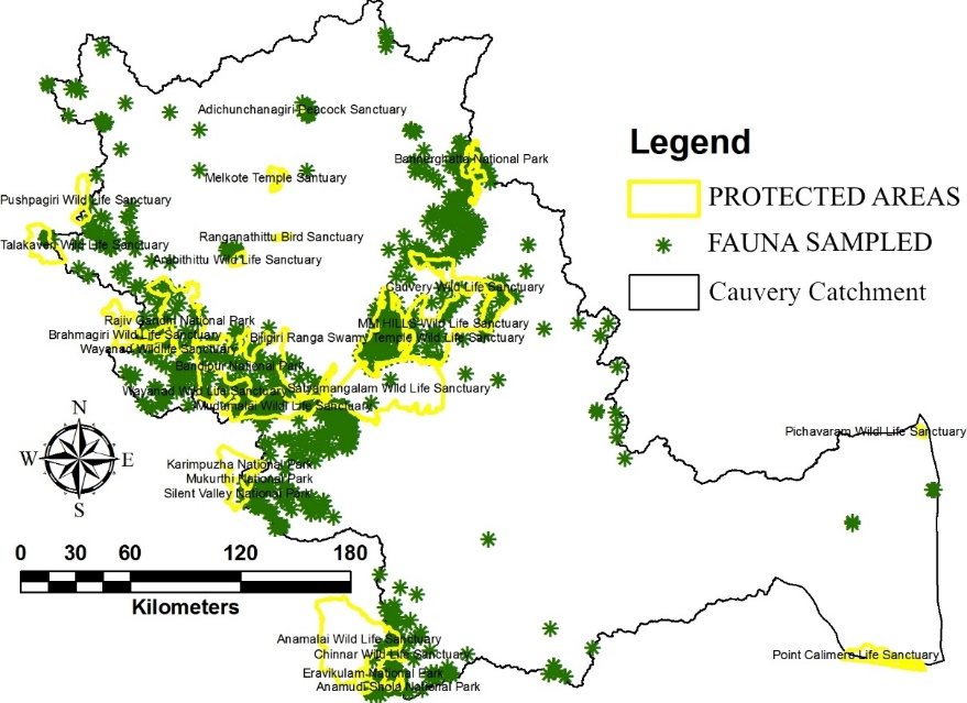 Figure 4.2.3: Faunal diversity of Cauvery basin PA
  Figure 4.2.4: Forest cover and PAs of Cauvery.
The following PAs fall with in basin, for which land use analysis has been carried out.
4.2.1 Pushpagiri Wildlife Sanctuary (PWLS):
Pushpagiri Wildlife Sanctuary is located in Somwarpet taluk of Kodagu district, Karnataka. PWLS adjoins Bisle reserve forest to the north and Kukke Subramanya forest range to the west. The topography of PWLS is dominated by steep terrains (160-1712 m) with waterfalls, swampy areas and streams. The rivers Lingadahole, Kumaradhara, Marigundhole and Uppangalhole flows through the sanctuary and acting as life line for the downstream population by the maintenance of ecological balance and soil and moisture conservation [3]. It has dense evergreen and semi-evergreen vegetation, with shola forests and grasslands in areas of higher elevation. It is one of the largest tropical evergreen forests in Karnataka with nearly 70% of the sanctuary covered with evergreen forests. The flora includes Artocarpus integrifolia, Artocarpus hirsuta, Artocarpus fraxinifolius, Alstonia scholaris, Calophyllum elatum, Calophyllum inophyllum, Calophyllum apetalum, Cedrella toona, Poeciloneuron indicum, Mesua ferrea, Palaquium ellipticum, Dipterocarpus indicus, Hardwickia binata, Vateria indica, Canarium strictum, Adina cardifolia, Syzigium cuminii, Lagerstromia lanceolate, Caryota urens, Antiaris toxicaria, Trewia nudiflora, Eugeniagardneri, Emblica officinalis, Terminalia peniculata, Terminalia chebula, Terminalia chebula, Terminalia belerica, Lagerstromia lanceolata, Xylia xylocarpa, Terminalia tomentosa etc. PWLS is rich in its fauna includes Asian Elephant, Lion tailed macaque, Indian Wild Dog, Brown Palm Civet, Indian Giant Squirrel, Indian Hare, Spotted Deer, Sambar, Gaur, Giant Flying Squirrel, Travancore Flying, Otter species, Stripe-necked mongoose, cobra, Indian rock python, king cobra and bamboo pit viper. The region has a rich diversity of birds (16 endemic endangered) such as Nilgiri wood-pigeon, grey-breasted laughing thrush, blue-winged parakeet, grey-headed bulbul, Malabar grey hornbill, black and orange flycatcher and Nilgiri flycatcher. The land use depicted in Figure 4.2.5 and Table 4.2.1 highlights status of vegetation cover from 1973 to 2016. The sanctuary has not shown any changes in its vegetation cover. But, the anthropogenic pressures due to commercial crops have transformed major forests in buffer region. The shift from agriculture to horticulture and from traditional forming to rubber, tobacco, coffee cultivation has impacted on flora and fauna as well as hydrological regime of entire region.
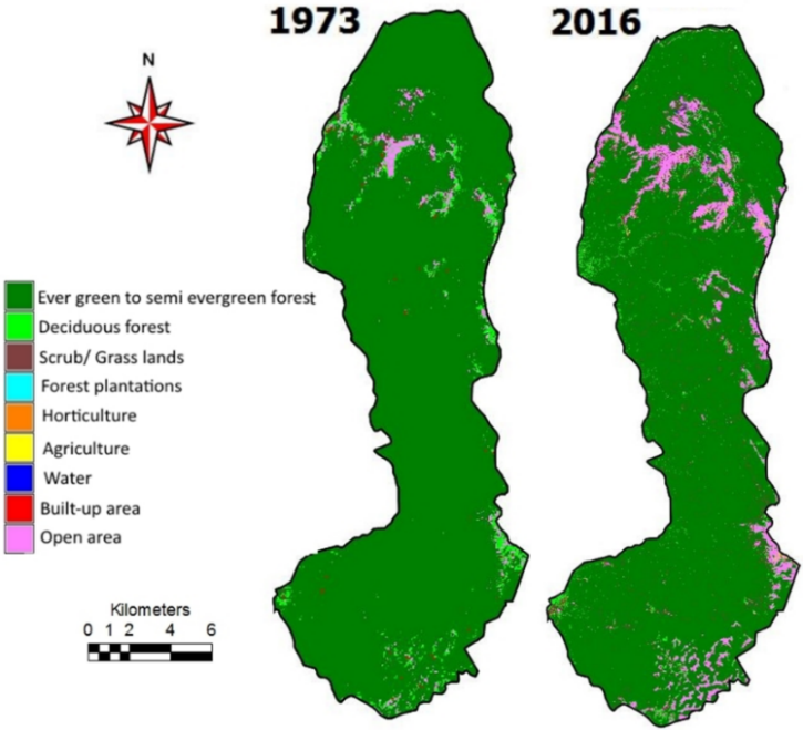
Figure 4.2.5: Land use analysis of PWLS.
Table 4.2.1: Temporal changes in land use
|
Category |
1973 |
2016 |
||
|
Ha |
% |
Ha |
% |
|
|
Ever green to semi evergreen |
80159.29 |
80.73 |
63841.17 |
64.29 |
|
Deciduous forest |
10110.33 |
10.18 |
13697.26 |
13.79 |
|
Scrub/Grass land |
693.65 |
0.70 |
5417.84 |
5.46 |
|
Forest Plantations |
87.5 |
0.09 |
524.12 |
0.53 |
|
Horticulture |
4089.87 |
4.12 |
6551.82 |
6.60 |
|
Agriculture |
613.05 |
0.62 |
2857.55 |
2.88 |
|
Water |
20 |
0.02 |
320.75 |
0.32 |
|
Built-up area |
37.79 |
0.04 |
133.88 |
0.13 |
|
Open area |
3485.43 |
3.51 |
5952.51 |
5.99 |
|
Total |
99296.91 |
|||
4.2.2 Talacauvery Wildlife Sanctuary (TWLS):
Talacauvery Wildlife Sanctuary is located in Madikeri taluk of Kodagu district of Western Ghats. It covers an area of 105.59 sq. km with lush evergreen and semi-evergreen type of vegetation all across because of high rainfall in the area while at the top of the hill sholas are present. Some part of this wildlife sanctuary also has moist deciduous forest. It is blessed with variety of floral (Dipterocarpus indicus, Antiaris toxicaria, Cinnamomum macrocarpum, Blachia umbellate, Artocarpus hirsutus, Pinanga dicksonii, Vateria indica, Pinanga dicksonii, etc.) and faunal species (Tiger, Leopard, Clawless Otter, Lion Tailed Macaque, Asian Elephant, etc.). This protected area is catchment for river Cauvery which originates from Talacauvery and the sanctuary also acts as an important catchment area for Perennial streams like Dodda Hole, Nadumale Hole, Betemale Hole, Kume Kolli and Mundra Hole. Land cover analysis for Talacauvery wildlife sanctuary for the year 1991 and 2016 is as shown in Figure 4.2.6, Table 4.2.2. The region has not witnessed any changes from 1991 to 2016 in its vegetation cover due to its high altitude forest and strict protection. Unlike core WLS the buffer region shows changes as increase in horticulture activities as a result of high rubber plantation, coffee plantations due to favorable rainfall. The existing agriculture regions were transformed for commercial plantations due to higher revenue opportunities. The deciduous forests near to existing settlements were transformed to rubber plantations and other commercial crops.
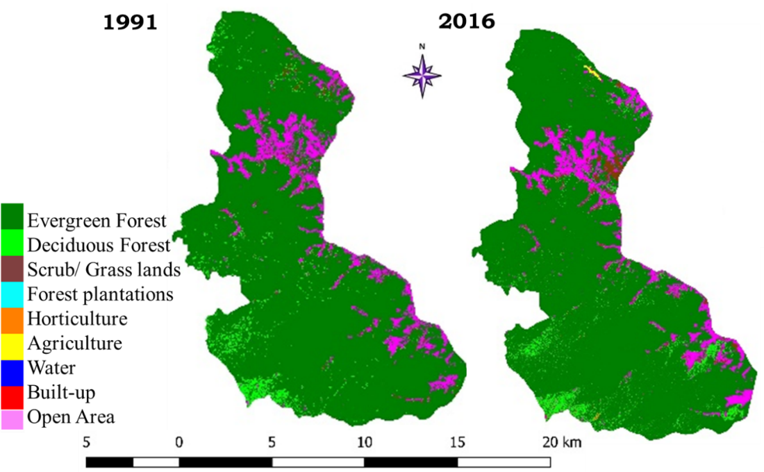
Figure 4.2.6: Land use of TWLS.
Table 4.2.2: Land use categories for the year 1991 and 2016
| Category |
1991 |
2016 |
||
|
Area (Ha) |
% Cover |
Area (Ha) |
% Cover |
|
|
Evergreen Forest |
10210.05 |
86.77 |
10015.96 |
85.55 |
|
Deciduous Forest |
385.29 |
3.27 |
441.311 |
3.77 |
|
Scrub Forest |
146.16 |
1.24 |
230.469 |
1.97 |
|
Forest Plantation |
0 |
0 |
0 |
0 |
|
Horticulture |
0 |
0 |
14.153 |
0.12 |
|
Agriculture |
0 |
0 |
10.173 |
0.09 |
|
Water Body |
0 |
0 |
0 |
0 |
|
Built Up |
3.15 |
0.03 |
0 |
0 |
|
Open Area |
1021.86 |
8.68 |
996.117 |
8.51 |
4.2.3 Brahmagiri Wildlife Sanctuary (BWLS):
Brahmagiri Wildlife Sanctuary (BWLS) is located in Kodagu district with mean annual rainfall of 2,500-6,000 mm. BWLS was notified in 1974 with a spatial extent of 181.29 sq. km covering two reserve forests-Brahmagiri and Urty. The region is undulating terrain (elevation ranging 65-1,607 m) with several steep valleys and hillocks. Eight rivers and streams originate in BWLS and flow into the Bay of Bengal (Laxmanthirtha, Ramthirtha and Kabini) and the Arabian sea (Borapole, Segamanihole, Somahole, Miugorehole and Urtihole). The vegetation types include evergreen and semi evergreen forests and shola grasslands in the higher elevations [4], [5]. Tree species in the evergreen forests consist of Cinnamonum zeylanicum, Cedrea toona, Alstonia scholaris, Artocarpus hirsutus, Callophyllum apetalum, Hydonocarpus laurifolia, Zanthoxylum rhetsa, Vitex altissima, etc. The semi-evergreen forests consist species of Terminalia, Diospyros, Holigarna, Ficus and Albizia. At low elevations, evergreen forests patches consist of species Dipterocarpus indicus, Kingiodendrum pinnatum, Humboldtia brunonis, etc. At medium elevations, evergreen to semi evergreen species - Mesua ferrea, Palaquium ellipticum Syzizium malabaricum, Olia dioca, Holigarna grahmii. Climbers include Entada phaseoloides, Spatholobus roxburghii, Calycopteris floribunda, Vetilago sp., Eleagnus sp. and Acacia pennata. This sanctuary is known for fauna - ~30 mammals including four species of primates, ~240 species of birds, etc. Among these 12 bird species (such as the blue-winged parakeet (Psittacula columboides) and small sunbird (Nectarinia minima) etc.) are Western Ghats endemic. The Brahmagiri-Pushpagiri area of the Talacauvery region has a total of 34-35 mammal species of which 14 are in the IUCN Red List threatened categories (including the lion tailed macaque and the Nilgiri langur) and six are endemic to India. Key flagship species of the Western Ghats such as Tigers (Panthera tigris) and Asian elephants (Elephas maximus), forests, occur in significant numbers. Other mammals include wild dog (Cuon alpinus), jungle cat (Felis chaus), Indian bison or gaur (Bos gaurus), sloth bear (Melursus ursinus) and wild pig (Sus scrofa), Deer species (chital or spotted deer (Axis axis), mouse deer (Moschiola meminna) and barking deer (Muntiacus muntjak)) are resident in BWLS. Among reptiles the draco or gliding lizard (Draco dussumieri), King cobra (Ophiophagus hannah), bamboo pit viper (Trimeresurus gramineus) and Malabar torrent toad (Ansonia oronata), an endangered amphibian, endemic to the Western Ghats found here.
BWLS is populated by tiny agricultural villages with coffee, cardamom and commercial plantations. Invasive species like Eupatorium, Chromolaena odorata and Lantana camara have affected the floral diversity of the sanctuary in the borders. Threats to the sanctuary are poaching, encroachments by coffee estates, firewood collection and hydroelectric projects. Human animal conflicts are noticed due to illegal collection of small timber, firewood, N.T.F.P., grass by villagers from within BWLS. The land use analyses for the period 1973 to 2016 in BGWLS region are given in Figure 4.2.7 and Table 4.2.3. The regions near the boundary and adjacent to major roads have undergone major transitions with commercial crop activities and monoculture plantations. The shift from traditional farming to commercial crop and intensified horticulture is noticed at very high rates in buffer areas.
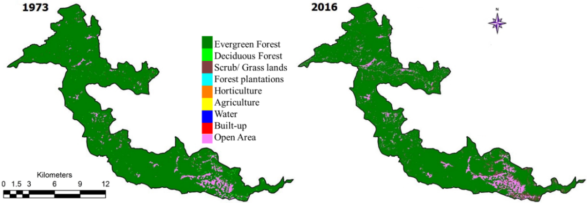
Figure 4.2.7: BWLS land use analysis.
Table 4.2.3: Land use of BGWLS from 1973-2016.
|
Category |
1973 |
1992 |
2016 |
|||
|
Ha |
% |
Ha |
% |
Ha |
% |
|
|
Ever green to semi evergreen |
17063.09 |
93.30 |
16538.49 |
90.43 |
16032.978 |
87.66 |
|
Deciduous forest |
132.21 |
0.72 |
205.01 |
1.12 |
285.09 |
1.56 |
|
Scrub/Grass land |
280 |
1.53 |
271.63 |
1.49 |
618.54 |
3.38 |
|
Forest Plantations |
0 |
0.00 |
0.9 |
0.00 |
1.6 |
0.01 |
|
Horticulture |
0 |
0.00 |
0 |
0.00 |
0 |
0.00 |
|
Agriculture |
0 |
0.00 |
0 |
0.00 |
0 |
0.00 |
|
Water |
0 |
0.00 |
|
0.00 |
8.305 |
0.05 |
|
Built-up area |
0 |
0.00 |
9.27 |
0.05 |
12.66 |
0.07 |
|
Open area |
813.69 |
4.45 |
1263.69 |
6.91 |
1329.82 |
7.27 |
|
Total |
18288.99 |
|||||
4.2.4 Bandipur National Park (BANP):
Bandipur national park (BANP) is located in Nanjungud and H.D. Kote taluks of Mysore district and Gundelpet taluk of Chamarajanagar district. BANP with a spatial extent of 872.24 sq. km, was notified in the year 2001 under section 35 (4) of Wildlife Protection Act, 1972 (amended in 2003). BANP has the distinction of getting Tiger Reserve status (1973), first among all national parks. Forest types include scrub (eastern most portion), dry deciduous (central portion), moist deciduous (western most part), etc. It harbors a wide variety of flora and fauna. The flora in the sanctuary are Shorea talura, Santalum album, Emblica officinalis, Terminalia chebula, Terminalia tomentosa, Chloroxylon swietenia, Lagerstroemia lanceolate, Dalbergia latifolia, Adina cordifolia, Acacia leucophloea, Odina wodiar, Butea monosperma, Acacia catechu, Tectona grandis etc. BANP is known for elephants, tigers, large guar¸ chital, sambar, jackal, leopard, porcupine, giant squirrel, sloth bear, mouse deer, etc. Reptiles include python, Indian monitor, rat snake, Russell’s viper, common cobra, etc. This region is a habitat for numerous bird species (~250 species) and Quails, Partridges and stone curlew, Malabar trogon, Malabar grey hornbill, Blue wing parakeet and White bellied minivet are endemic to Western Ghats.
The park receives pre-monsoon showers, South-West monsoon and North-East monsoon, average rainfall varies from 914 mm to 1270 mm. Two national highways connecting Mysore-Ooty and Mysore-Calicut passes through the park. There has been frequent cases of natural and man-made forest fires within the wildlife sanctuary. Fire impact assessments based on online web portals BHUVAN [6] reveal that about 2627.707 Ha (2.8%) was severely impacted by fire disaster. Rampant habitat degradations were due to unplanned developmental projects such as dams and interstate highways in the ecologically sensitive habitats apart from other pressures such as grazing, firewood collection and weed infestation (Eupatorium, Parthenium, Chromolaena odorata), illegal hunting, poaching (elephant poaching for ivory), etc. [7]. due to lack of effective eco-management leading to a very frequent instances of human-animal conflicts. Unauthorised occupation of forest lands for cultivation in the buffer region has aggravated human-animal conflicts leading to the frequent death of animals. Elephants killed in conflicts (electrocution, hunting, road accidents) are 39 during 2007-2012, which highlights the seriousness of the conflict. Land use analysis is shown in Figure 4.2.8 and Table 4.2.4 reveal a decline of 15.19 % forest cover. Eastern portions of the park have under gone major transition due to fire and anthropogenic disturbances. Native deciduous forest is converted into scrub forests (8 to 23.11 %), infested by exotic weeds, with the enhanced cattle grazing, agricultural activities
. Table 4.2.4: Land use analyses of BANP
|
Category |
1973 |
2016 |
||
|
Ha |
% |
Ha |
% |
|
|
Evergreen Forest |
183.6 |
0.2 |
15.08 |
0.02 |
|
Deciduous Forest |
84569.04 |
90.04 |
70311.56 |
74.85 |
|
Scrub Forest |
7992.72 |
8.51 |
21713.87 |
23.11 |
|
Forest Plantation |
0 |
0 |
64.77 |
0.07 |
|
Horticulture |
0 |
0 |
7.68 |
0.01 |
|
Agriculture |
801 |
0.85 |
767.53 |
0.82 |
|
Water Body |
367.92 |
0.39 |
353.28 |
0.38 |
|
Built-Up |
0 |
0 |
53.83 |
0.06 |
|
Open Area |
12.24 |
0.01 |
651.49 |
0.69 |
|
Total |
93926.52 |
|||
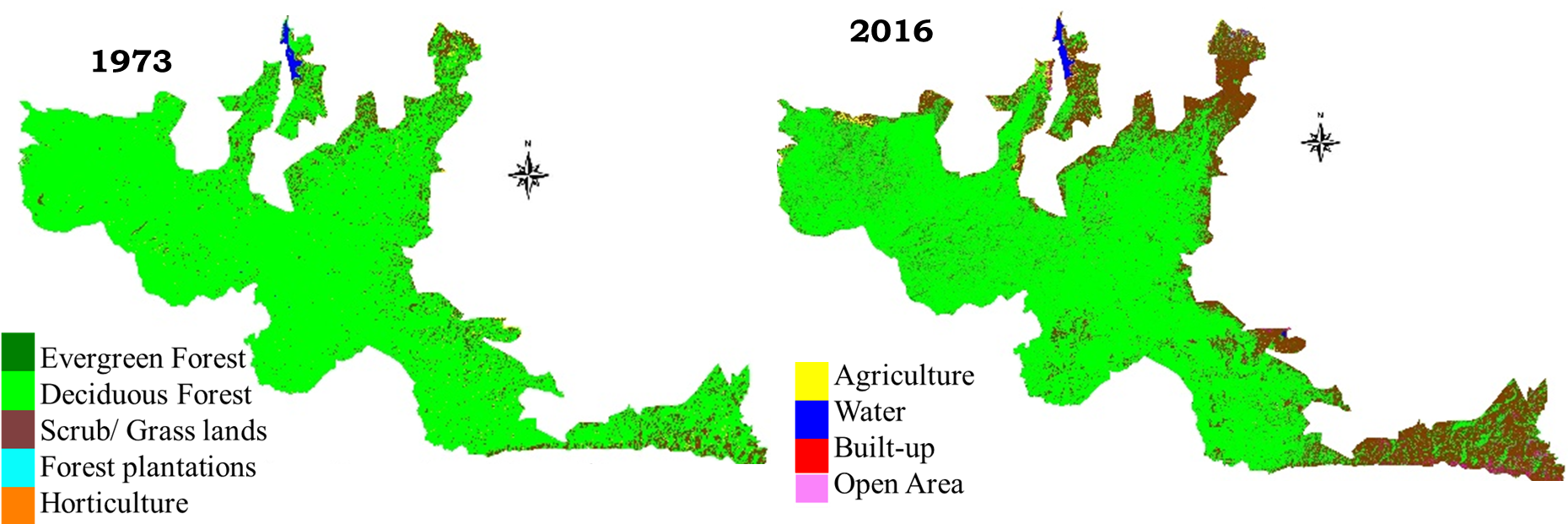
Figure 4.2.8: Temporal changes in BANP.
4.2.5 Nagarholé National Park (Rajiv Gandhi Tiger Reserve):
Nagaraholé national park is located in the district of Mysore and Coorg of Karnataka state and also part of the Nilgiri biosphere reserve. It can be considered as the cultural landscape that reflects the historical, socio-economic relationship of humans and places. It has derived its name due to the stream (Holé) which is in the shape of cobra (Naga). It is also known as Rajiv Gandhi Tiger Reserve-RTR covering an area of 643.39 sq. km in 1974. The park was declared the 37th project tiger reserve in 1999 and was notified under section 35 (4) of WPA, 1972 (amended 2003) (Final notification) in 2003. RTR shares its boundaries with Bandipur wildlife sanctuary which together is a part of Mudumalai Sanctuary in Tamil Nadu and the Wayanad reserve in Kerela and are the best protected habitats for endangered species such as elephants and tigers. The park mainly consists of moist deciduous forest in the Northern and Western part and dry deciduous in the south-eastern part. Plantations of teak, bamboo, rosewood, eucalyptus, sandalwood are present in the park. Some of the dominant floral species present in the sanctuary are rosewood, teak, sandalwood, silver oak, ficus, cotton tree, kadam, mathi (Terminalia tomentosa), nandi (Lagerstroemia lanceolata), hone (Pterocarpus marsupium), etc. The park also has a variety of faunal species like tiger, elephant, leopard, sloth bear, hyena, deer, slender loris, giant flying squirrel, porcupine, etc. Bird species present are racket tailed drongo, stork billed, kingfisher, woodpeckers, blyth’s baza, peregrine, cuckoos, teals, ibis, etc. There is a variety of reptile species as well consisting of monitor lizard, vine snake, python, Russell’s viper, crocodiles, etc.
Some of the major problems in the National park is unabated poaching activities, escalating human-animal conflicts, frequent fires (due to natural and anthropogenic sources), invasion of weeds, smuggling of timber, increase in human habitations, etc. Tribal population of 6000-7000 inhabit the national park and the villages fringing NNP have witnessed increase in population. These villagers rely on the forest for grazing, fuelwood and timber collection. There are reports of killing of 77 elephants in the park during January, 2000 to October, 2002. The park also suffers from forest fires on regular basis. In 2004 also there was a huge fire in the park burnt around 40 hectares of forest area. Figure 4.2.9 and Table 4.2.5 highlights the status of vegetation cover during 1973 to 2016. The analysis reveals a decline of 11 % forest cover due to increase in human activities within the national park and in the buffer region. The buffer region is highly dominated by horticulture activities and grazing. There is a slight increase in scrub forest, rosewood, teak plantations.
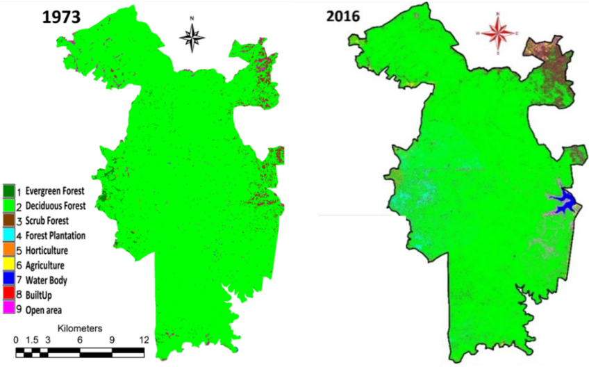
Figure 4.2.9: Land use changes in RTR.
Table 4.2.5: Land use of RTR from 1973-2016
| Category |
1973 |
2016 |
||
|
Ha |
% |
Ha |
% |
|
|
Ever green to semi evergreen |
598.77 |
0.88 |
311.19 |
0.46 |
|
Deciduous forest |
65470.41 |
96.06 |
58,589.84 |
85.99 |
|
Scrub/Grass land |
1474.11 |
2.16 |
4490.878 |
6.59 |
|
Forest Plantations |
0 |
0 |
2,210.08 |
3.24 |
|
Horticulture |
59.76 |
0.09 |
207.13 |
0.3 |
|
Agriculture |
0 |
0 |
666.24 |
0.98 |
|
Water |
21.87 |
0.03 |
383.34 |
0.56 |
|
Built-up area |
0 |
0 |
14.113 |
0.02 |
|
Open area |
508.32 |
0.75 |
1259.328 |
1.85 |
|
Total |
68133.24 |
|||
4.2.6 Biligiriranganatha Swamy Temple (BRT) Tiger Reserve:
BRT (Biligiriranganatha Swamy Temple) Wildlife Sanctuary is located in the Yelandur, Kollegal and Chamarajanagar taluks of Chamarajanagar district. It covers an area of 539.52 sq. km. It was declared as a Tiger Reserve in January, 2011 by the Government of Karnataka acts as a corridor between Eastern Ghats and Western Ghats. It is nurtured by river Cauvery and river Kollegal. BRT WLS has a total of around 800 species of plants which shows many resemblance towards Western Ghats such as Anogeissus latifolia, Dalbergia paniculata, Baswellia serrata, Commiphora caudate, Acacia chundra, Diospyros melanoxylon, etc. BRT is also famous for its rich faunal species such as elephants, tigers, Indian gaurs, leopards, wild dogs. The sanctuary amounts to a total of 713 elephants in 610 km2. Apart from these, it has a wide variety of butterflies, reptiles, insects and birds. The Soligas are an indigenous tribal community of BRT, approximately 6000 Soligas live in forest villages called podus (tribal settlements). Traditionally, the Soligas were hunters and shifting cultivators and collected a wide range of non-timber forest products (NTFP). There are many human enclaves inside the sanctuary, including settlements of indigenous people, temple staff, and private estates of commercial plantations growing coffee (Coffea Arabica), pepper (Piper nigrum), cardamom (Elettaria cardamomum) etc. [8]. Figure 4.2.10 shows land use analysis of BRT wildlife sanctuary and Table 4.2.6 depicts the land use categories area. It can be seen that evergreen forest and deciduous forest cover has declined over years and there is a sharp increase in the scrub forest due to deforestation in the edges. Reduction in forest cover is also due to increase in illegal encroachment by the natives within the boundary.
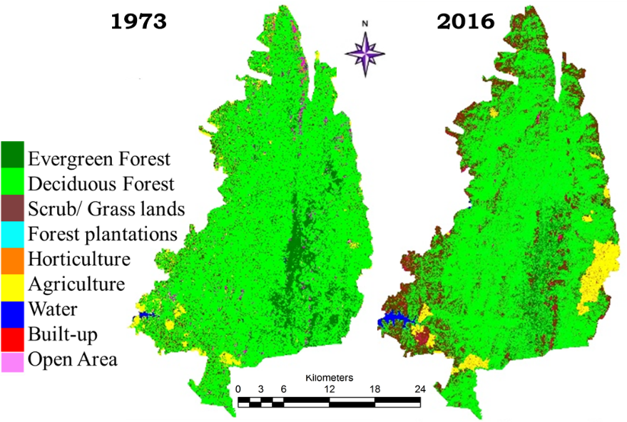
Figure 4.2.10: BRT region temporal land use
Table 4.2.6: BRT Wildlife Sanctuary land use details
|
Category |
1973 |
1991 |
2016 |
|||
|
Ha |
% |
Ha |
% |
Ha |
% |
|
|
Evergreen Forest |
7533 |
11.5 |
6994.62 |
10.68 |
2837.9 |
4.33 |
|
Deciduous Forest |
48984.48 |
74.79 |
47390.94 |
72.36 |
42748.93 |
65.27 |
|
Scrub Forest |
4804.2 |
7.33 |
6500.97 |
9.93 |
14691.26 |
22.43 |
|
Plantation |
0 |
0 |
0 |
0 |
764.445 |
1.17 |
|
Horticulture |
742.32 |
1.13 |
120.78 |
0.18 |
265.898 |
0.41 |
|
Agriculture |
1832.04 |
2.8 |
3359.07 |
5.13 |
2688.493 |
4.1 |
|
Water Body |
115.92 |
0.18 |
195.57 |
0.3 |
365.8 |
0.56 |
|
Built-Up |
0 |
0 |
17.55 |
0.03 |
498.143 |
0.76 |
|
Open Area |
1485.36 |
2.27 |
918.09 |
1.4 |
636.358 |
0.97 |
|
Total |
65498.22 |
|||||
4.2.7 M.M. hills Wildlife Sanctuary (MMHWLS):
Malai Mahadeshwara wildlife sanctuary is located in the Eastern Ghats in Kollegal taluk of Chamarjanagar district, located very close to tri-junction of the states of Karnataka, Tamil Nadu and Kerala. The wildlife sanctuary was established in the year 2013 and was notified under section 26 A (1) (b) of Wildlife Protection Act, 1972 as (amended up to 2003) (final notification) with an area of 906.18 sq. km. The sanctuary has Cauvery wildlife sanctuary to its North and East, Sathyamangalam wildlife sanctuary to its South and BRT Wildlife Sanctuary to its west. The predominant vegetation type of the sanctuary is dry and moist deciduous forests. The floral species found in the sanctuary are Anogeissus latifolia, Boswelia serrata, Chloroxylon swietinia, Den drocalamusstrictus, Pterocarpu smarsupium, Tectonagrandis and Terminalia. Faunal species include tiger, leopard, striped hyena, sloth bear, elephant, gaur, chital, four horned antelopes, otter, marsh crocodile. MMHWLS forms an important part of the savannah woodland forests of Karnataka and also forms part of the Mysore Elephant Reserve declared by Project Elephant which supports good densities of Asian elephants depicting the ecological importance of the sanctuary and recently tigers have also been documented in this wildlife sanctuary. Increased degradation of forest resulted in drought condition, s led to death of many animals in the region. Cases of animals dying due to consumption of contaminated water are noticed (FIAPO, 2013). Land use analysis was done to obtain more insights in landscape dynamics as shown in Figure 4.2.11 and Table 4.2.7. There is no significant reduction in the evergreen forest while deciduous forest has significantly declined by 11.83% from the year 1973 to 2016 and converted into scrub forest. (14.05 %).
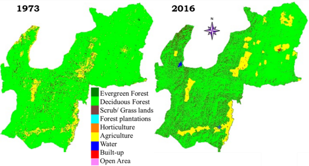
Figure 4.2.11: Temporal change in land use of MM Hills.
Table 4.2.7: Land use analyses for MM Hills
|
Category |
1973 |
2016 |
||
|
Ha |
% |
Ha |
% |
|
|
Evergreen Forest |
205.56 |
0.21 |
162.90 |
0.17 |
|
Deciduous Forest |
87357.60 |
88.58 |
75691.61 |
76.75 |
|
Scrub Forest |
3041.28 |
3.08 |
13857.86 |
14.05 |
|
Forest plantation |
0 |
0 |
0 |
0 |
|
Horticulture |
2.16 |
0 |
11.15 |
0.01 |
|
Agriculture |
7753.68 |
7.86 |
8285.97 |
8.4 |
|
Water Body |
35.64 |
0.04 |
184.12 |
0.19 |
|
Built-Up |
3.96 |
0 |
195.92 |
0.2 |
|
Open Area |
216.72 |
0.22 |
234.80 |
0.24 |
|
Total |
98616.60 |
|||
4.2.8 Cauvery Wildlife Sanctuary (CWLS):
The Cauvery wildlife sanctuary (CWLS) is located on the banks of the river Cauvery with an area of 1027.53 sq. km in district of Chamarajanagar, Ramnagar and Mandya of Karnataka. It was established in the year 1994, notified under the section 26 (A) (b) of Wildlife Protection act, 1972 as (amended 2003). CWLS forest types include dry deciduous type and some portion is moist deciduous and scrub forest. The predominant species of flora are Hardwickia binate and Albizzia amara, Wrightia Tinctoria, Azadirachta indica, Tamarindus indica, Vitex altissima, Emblica officinalis, Acacia leucophloea, Acacia sundra, Terminalia arjuna, Pongamia glabra, Vitex altissima, Eugenia jamboolina, etc. CWLS harbors a wide variety of faunal species such as Elephant, Tiger, Gaur, Leopard, Four horned antelope, Mouse deer, etc. River Cauvery passes through the sanctuary and supporting a variety of aquatic fauna such as crocodiles, otters and Mahseer fish. There are various threats to the wildlife sanctuary such as poaching, grazing, encroachments, deforestation, illegal timber collection, smuggling of forest goods etc. The poaching of wild animals for commercial benefits is major problem due to higher density of population in and around. Poaching of bull elephant is common for ivory. The hunting of wild boars, sambar, deer, hares for meat and catching fishes for domestic consumption by villagers cannot be ruled out. There are 30 villages within the radius of 5Km having population of humans 35000 and cattle of 39000. The problem of encroachment is mainly because of the increase in population in and around the sanctuary which has led to increasing demand of agricultural land. The river Cauvery serpentine through the hills encloses many places of tourist interest and religious importance. Mekedhatu and Hogenakal falls are noted tourist spots while Muthathu is a place of revered religious importance. The vegetation cover has lost though strict protection is enforced due to population pressure and encroachments. The area under vegetation has declined by 18.43% during 1973-2016 as shown in Figure 4.2.12 and Table 4.2.8. There is an increase in agricultural, horticulture practices and loss of the water bodies. All these changes signify that there is an increased human intervention due to population present within the sanctuary. Also overgrazing is another problem in this wildlife sanctuary resulting in denudation of grassy patches. It can be seen that there is a huge decline in the deciduous forest and a significant rise in the scrub forest. The agricultural activities have increased portrays increase in human population in the buffer region led to conversion of the forest into scrub forest by over exploitation. The uncontrolled grazing and mismanagement of gomala lands (revenue lands reserved for grazing) forcing population to intrude in forest area.
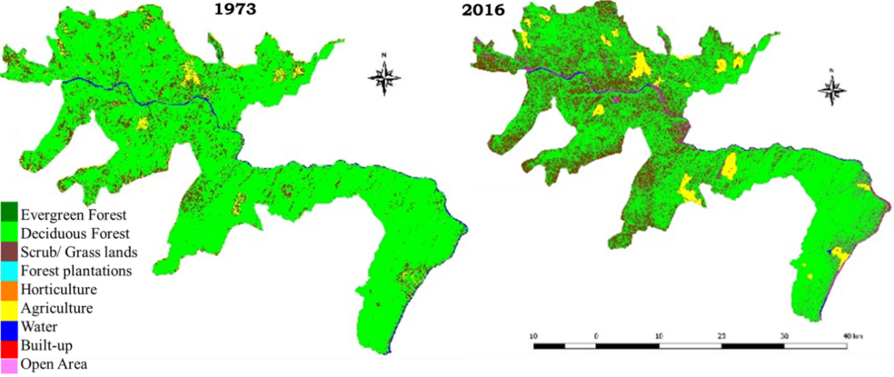
Figure 4.2.12: Temporal land use of CWLS.
Table 4.2.8: Change in land use pattern of CWLS from 1973-2016.
|
Category |
1973 |
2016 |
||
|
Ha |
% |
Ha |
% |
|
|
Evergreen Forest |
0 |
0 |
0 |
0 |
|
Deciduous Forest |
94107.24 |
85.73 |
74025.96 |
67.43 |
|
Scrub Forest |
11521.08 |
10.5 |
26891.45 |
24.49 |
|
Plantation |
0 |
0 |
0 |
0 |
|
Horticulture |
0 |
0 |
13.48 |
0.01 |
|
Agriculture |
2779.92 |
2.53 |
4540.5 |
4.14 |
|
Water Body |
1314 |
1.2 |
747.63 |
0.68 |
|
Built-Up |
0 |
0 |
335.86 |
0.31 |
|
Open Area |
48.6 |
0.04 |
3229.82 |
2.94 |
|
Total |
109770.84 |
|||
4.2.9 Bannerghatta National Park (BNP):
Bannerghatta National Park (BNP) was declared as national park in 1974 with an area of 106.83 sq. km. The various plans and proposals were considered by forest department, Government of Karnataka till 2009 to widen and develop the Bannerghatta National Park. These plans were created for reducing the pressure of the people residing in the periphery of the park, reducing human-animal conflict as well as depredation of crop by elephants, habitat improvement for increasing the carrying capacity of the park and the restoration of entire ecosystem. The total area of BNP now encompasses an area of 260.51 sq.km comprising of 13 reserve forests spread over the districts of Bangalore urban, Bangalore rural and Ramanagara as per Vide G. O. No. FEE 302 FWL 2011 (II), dated: 27.12.2011. The boundary of BNP is having highly irregular shape and it measures about 59 km in length and the width varies from 0.3 km to 13.8 km. BNP is situated close proximity to Bangalore metropolitan city (20 km to the BNP core area and 1.8 km from Bruhat Bengaluru Mahanagara Palike (BBMP) boundary), capital state of Karnataka. The encroachment of forests, stone quarrying, sand mining and domestic livestock grazing are the major threats of BNP region. Unabated activities of quarries are causing disturbance to wild animals due to use of explosives, and movement of vehicles and also disturbance to the park authority as they are illegal and needs to be stopped. BNP experiences high grazing pressure due to the concentration of livestock population in the surrounding villages is another major problem in the northern and western boundaries.
Land use changes within BNP region are shown in Figure 4.2.13 and Table 4.2.9. The moist deciduous forest was covered 50.4% (1973) and now 28.5 % (2015) due to anthropogenic pressure in BNP and its environs. The BNP region has increase in agriculture area from 7.62 to 13.6 % by 2015. Forests in Ragihalli, Manjunatha, Yelavantha, Bettahalli regions with good protection measures show minimal disturbance. However, implications of unplanned urbanization are evident in the buffer regions. Land use analysis highlights of urban sprawl in peri-urban regions has fragmented, dispersed urban patches in periphery accounting to 5462 ha (built-up area). The region has 9254.21 ha of scrub forests and which can be reforested for better protection of ecosystem in BNP. The western and eastern part of the BNP and buffer region are composed of agricultural village communities. There is a predominance of sugar cane, ragi, eucalyptus in the eastern part; paddy, coconut and mango plantations in the western part. The large tracts of deciduous cover in Kanakapura taluk, Anekal taluk region are lost due to intensification of horticulture area in recent years and consequent land use changes. Urbanization in the vicinity of ecologically sensitive national park highlights the extent of unplanned senseless urbanization (in the form of housing layouts, etc.) and also mirrors the extent of fragmented governance. BNP is vital for Bangalorean’s as it helps in moderating climate, sequester carbon, oxygen production and wide array of flora of medicinal importance [9]. The conservation of this region requires instantaneous inventorying, mapping and monitoring of biological resources.
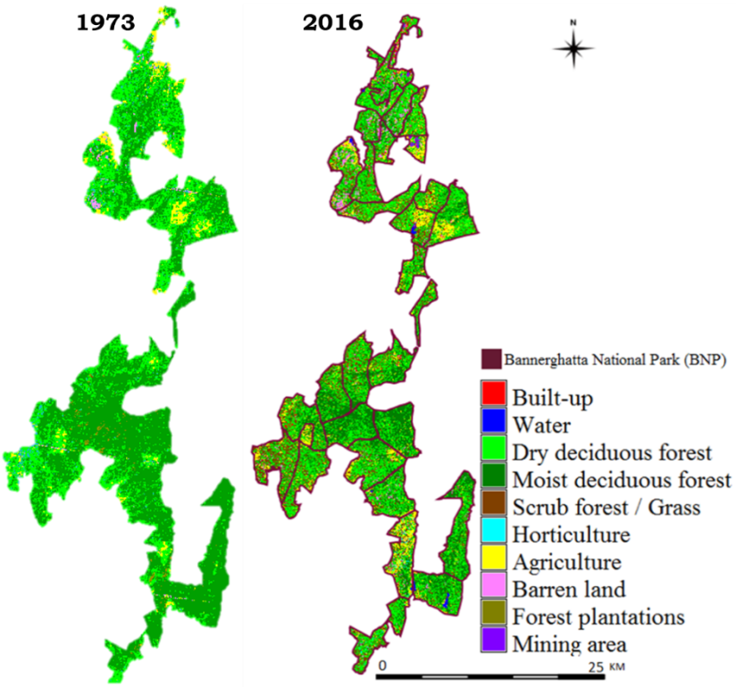
Figure 4.2.13: Land use changes of BNP region.
Table 4.2.9: Land use of BNP from 1973-2015.
|
Category |
1973 |
1989 |
2015 |
|||
|
Ha |
% |
Ha |
% |
Ha |
% |
|
|
Dry deciduous forest |
32415.6 |
26.6 |
31609.3 |
26.0 |
22729.9 |
18.7 |
|
Moist deciduous forest |
31725.9 |
26.1 |
29694.3 |
24.4 |
16822.2 |
13.8 |
|
Grass/Scrub forest |
4876.8 |
4.0 |
4500.4 |
3.7 |
9254.2 |
7.6 |
|
Water |
377.8 |
0.3 |
922.5 |
0.8 |
1834.0 |
1.5 |
|
Horticulture |
10361.3 |
8.5 |
11768.4 |
9.7 |
13363.2 |
11.0 |
|
Agriculture |
36027.9 |
29.6 |
37222.3 |
30.6 |
45613.8 |
37.5 |
|
Urban |
490.6 |
0.4 |
581.6 |
0.5 |
5462.1 |
4.5 |
|
Barren land |
4461.8 |
3.7 |
4251.7 |
3.5 |
3536.6 |
2.9 |
|
Forest plantations |
921.4 |
0.8 |
1060.5 |
0.9 |
1566.3 |
1.3 |
|
Mining area |
61.8 |
0.1 |
109.9 |
0.1 |
1538.7 |
1.3 |
|
Total |
121720.9 |
|||||
4.2.10 Adichunchanagiri Peacock Sanctuary (APS): Adichunchanagiri Peacock Sanctuary is situated in Nagamangala taluk of Mandya district in Karnataka notified under section 18 of Wildlife Protection Act, 1972 as (amended in 2003) (Final Notification) in 1981. It covers an area of 0.84 km2. The sanctuary is located near Chunchanagiri Temple and is a typical hill having giant tors heaped up by various boulders. There is good number of peafowls in the sanctuary due to high protection put in effect with strong religious sentiments. The sanctuary is dominated by southern thorn scrubs and some exotic species such as Eucalyptus tereticornis and Acacia auriculiformis which were introduced in past. The native vegetation in the region is mostly denuded. Some of the species found here are Annona squamosa, Andrographis serpellyforlia, Lagascea molis, Tecoma stans, Ficus religiosa, Cycas circinalis, etc. The sanctuary as well as other nearby hills have good number of peafowls. Some of the fauna found are Bonnet Macaque, Pipistrelle, Flying fox, Black naped hare, Little grebe, Grey pelican, Lesser whistling teal, Tawny eagle, Scavenger vulture, Koel, Paraiah kite, Brahminy skink, Fanthroated lizard, Crimson rose, Common mormon, The pioneer, etc. The sanctuary has 17 villages at the fringes with a population of about 11980. It is surrounded by coconut plantations and agricultural fields. Nearly 50000-75000 pilgrims visit the temple on festive occasions which causes some disturbance. Another problem is occasional illegitimate cutting of eucalyptus trees.
Land use analysis (Figure 4.2.14) depicts major portion of the sanctuary under scrub forest cover and open areas as shown in Table 4.2.10. The scrub forest covers 61.87 % major region prone to grazing due to lack of grassy patches in the surrounding villages.
|
|
|
|||||||||||||||||||||||||||||||||||
|
Figure 4.2.14: Land use (2016) of APS |
Table 4.2.10: Land use area details of APS |
|||||||||||||||||||||||||||||||||||
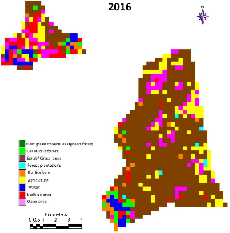
4.2.11 Arabithittu Wildlife Sanctuary:
Arabithittu Wildlife Sanctuary is situated in Hunsur taluk of Mysore district of Karnataka and cover a latitude range of 12º 17’ 16” to 12º 20’ 41” North and longitude range of 76º 22’ 43” to 76º 28’ 51” East. The extent of this sanctuary is 13.50 km2. The sanctuary is surrounded by agricultural fields by all the sides except for North eastern region (belongs to Defence area). Elephants from Nagarahole National Park have been reported in this sanctuary. The sanctuary is surrounded by 87 villages having a population of 3.5 lakhs. The mean annual rainfall in this region is around 800 mm and the temperature varies from 17.8º-35º C. The forest is of dry deciduous scrub type and has large amount of Sandalwood trees, other species found in the region are Cassia fistula, Chloroxylon swietenia, Pterocarpus marsupium, Kydia calycina, Albizia amara, Ficus benghalensis, Bauhinia racemose, Albizia lebbeck, Bombex ceiba, Emblica officinalis, Lagestroemia microcarpa, Ficus racemose, Tectona grandis, Ficus religiosa, Syzygium cumini, Diosphyros melanoxylon, Mangifera indica, Mitragyna parviflora, Santalum album, etc. The region is slowly improving in the native vegetation which acts as a favorable habitat for various faunal species. The sanctuary harbors good variety of faunal species such as Leopard, Wild boar, Common mongoose, Spotted deer, Partridges, Black drongo, Cobras, Vipers, etc. The region has not been recorded with any poaching or hunting activities. There are not much cases of illegal cutting of trees except wounding of eucalyptus plantations is recorded during tobacco cultivation. Major problem is cattle from the nearby villages are left loose to graze within the forest.
Land use analysis (Figure 4.2.15, Table 4.2.11) shows major forest cover is under scrub and grass land forest types (52.75 %), followed by deciduous cover (34.54 %) supporting herbivorous fauna effectively. The region is acting as a temporary halt for various faunal species such as Elephants migrating from Nagarholé (RTR) to other places. The agriculture shows 9% represents anthropogenic status in the region. Eucalyptus plantations in the sanctuary and its surrounding are degrading natural cover over a decade, interventions are the need of the hour to control it.
|
|
|
|||||||||||||||||||||||||||||||||||
| Figure 4.2.15: Arabithittu Wildlife Sanctuary Land use status | Table 4.2.11: Land use area details of Arabithittu Wildlife Sanctuary | |||||||||||||||||||||||||||||||||||
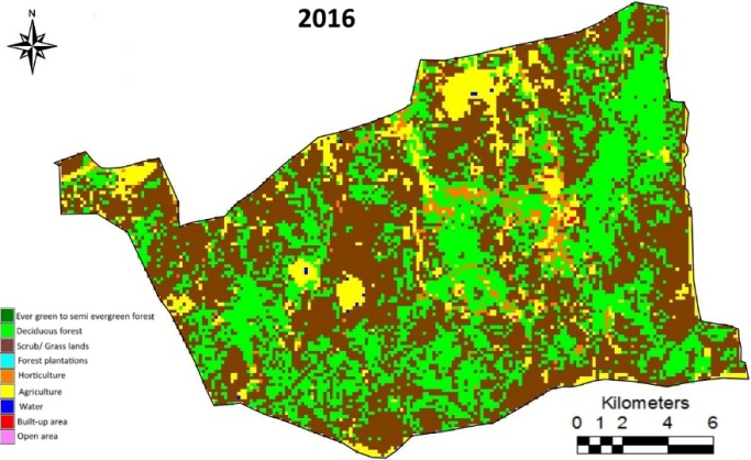
4.2.12 Melkote Wildlife Sanctuary:
Melkote Wildlife Sanctuary is situated in Mandya district of Karnataka, spread in two blocks: Narayandurga (45.34 km2), Mudibetta (4.48 km2) covering a total area of 49.82 Km2. It is extended from latitudinal range of 12º 37’ to 12º 44’ North to Longitudinal range of 76º 34’ to 76º 40’ East. It was notified under section 18 of Wildlife Protection Act, 1972 as (amended in 2003) (Final Notification) in 1974. The annual average precipitation in the region is 621 mm and the temperature ranges from 17º-38º C. The vegetation in the region is dominated by tropical dry deciduous species along with scrubs and rocky outcrops. Some of the major floral species found in the region are Terminalia chebula, Angogeissus latifolia, Chloroxylon swietenia, Acacia leucophloea, Santalum album, Zizyphus sp., etc. The region also has Cycas circinalis which is an endangered species of gymnosperm. The sanctuary also has a good faunal diversity such as Wolf, Jungle cat, spotted deer, Leopard, Bonnet macaque, Black buck, Langur, Pangolins, etc. The region also harbors a variety of butterflies, birds and reptiles. Around 110 species of butterflies and 199 species of birds are present in the sanctuary.
The sanctuary was specifically declared to protect Grey wolves. The major problem in the region is disappearance of wolves and black bucks. Forest department earlier planted some fast growing native as well as exotic tree species such as eucalyptus, etc., which has replaced the original scrub forest type. This has led to leopard taking over the forest and wolves entering the fields being killed by humans. There are not much open fields left for blackbucks and antelopes which has led to reduction in their population (Suresh, 2012). Land use analysis (Figure 4.2.16, Table 4.2.12) shows major cover is under scrub/ grass lands and deciduous forest. Frequent human induced forest fires in the grass lands has caused impact on regeneration of natural vegetation, which has resulted in proliferation of exotic weeds. The creation of water holes and grassy patches are to be done as priority management activity to control depredation of crops by wild animals in and around the sanctuary.
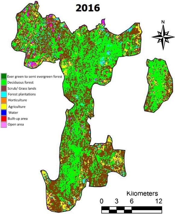
|
|
|||||||||||||||||||||||||||||||||||
| Figure 4.2.16: Melkote WLS land use status | Table 4.2.12: Land use analysis of Melkote WLS | |||||||||||||||||||||||||||||||||||
4.2.13 Ranganathittu Bird Sanctuary:
Ranganathittu Bird Sanctuary is a part of Srirangapatna taluk of Mandya district in Karnataka. It is extended across an area of 0.67 km2. It is located at 12º 25’ North and 76º 39’ East. The preliminary notification of the sanctuary was notified under section 4 (b) of Mysore Game and Preservation Act in 1940, Later in 1998, final notification came and it was notified under section 26 A (1) (a) of Wildlife Protection Act, 1972 as (amended in 2003). The region receives an annual rainfall of 700-800 mm during the month of June-October and average temperature of the region ranges from 15º-30º C. The region has thorny scrub jungles along with broadleaf deciduous forest. The region harbors around 400 species of plants belonging to 79 families. Some of the scrubby vegetation species found here are Dichrostachys cinerea, Pterolobium hexapetalum, Acacia sp., Capparis sp., etc. and the broad-leaved tree species in the region includes Terminalia arjuna, Syzigium cumini, Vitex leucoxylon, Barringtonia racemosa, Ailanthus excels, etc. Some of the other species found in the region are Iphigenia mysorensis, Cassia auriculata, Dodonaea viscosa, Hardwickia binata, Gymnema sylvestre, Marsdenia volubilis, Ichnocarpus frutescens, Cassytha filiformis, Hydrocotyle conferta, Pandanus fascicularis, Limonia acidissima, Aegle marmelos, Caralluma, Opuntia, Centella asiatica, Spilanthes calva, Alternanthera sessilis, Cryptocoryne retrospiralis, Eclipta alba, Hydrilla verticillata, Vallisneria spiralis, Lemna perpusilla, etc. The region also harbors some of the medicinal plant species such as Asparagus racemosus, Hybanthus enneaspermus, Hemidesmus indicus, Trichodesma indicum, Tinospora cordifolia, etc. The region also has some non-flowering plants such as Horsetail fern, Azolla pinnata, Marsilea minuta, etc. The sanctuary is a home to wide variety of fauna as it has such a diverse vegetation. There are around 221 species of birds belonging to 61 families including both resident and migratory. Some of them are White ibis, Herons, Egrets, Open billed stork, Spoonbill, Cliff sparrow, Great stone plover, Kingfishers, Grey partridge, Wattled lapwing, Pipits, Quails, Flycatcher, Warblers, Eagles, Kite, Owls, Whistling teal, Rosy pastor, Sand piper, Bronze winged jacana, Pied crested cuckoo, Redheaded bunting, etc. The sanctuary is also a home for various mammals (Common mongoose, Bonnet macaque, Common otter, Fruit bat, etc.), reptiles (Snakes, Common Indian monitor, Turtles, Marsh crocodiles, etc.), arthropods (61 species of Butterflies, Spider, Crabs, Centipedes, Mites, Crickets, Dragonflies, Damselflies, Termites, Bugs, Cicadas, Water scorpions, Ant lions, Beetles, Wasps, Bees, Ants, etc.). The sanctuary is surrounded by 24 towns and villages and have a cattle population of 67228. Even though there is no direct access to the islands, during summer or when water is low, cattle tend to enter the islands and damage the saplings disrupting regeneration. Land use analysis (Figure 4.2.17, Table 4.2.13) of the region shows 20 % area under horticulture helping the birds to nest and people are also protecting the birds without disturbing. The deciduous covers of 12.84 % dominated by trees such as tamarind, neem etc., are also helping the birds to nest. The region has some grass patches supporting as a prey base for birds.

|
|
|||||||||||||||||||||||||||||||||||
| Figure 4.2.17: Land use of Ranganathittu Bird Sanctuary | Table 4.2.13: Ranganathittu Bird Sanctuary land use status. | |||||||||||||||||||||||||||||||||||
4.2.14 Ramadevara Betta Vulture Sanctuary:
Ramadevara Betta Vulture Sanctuary is located in Ramanagara district of Karnataka. It is extended from 12º 44’ 21.70” to 12º 45’ 50.75” North and from 77º 17’ 20.27” to 77º 18’ 45.63” East covering an area of 3.46 Km2. It was notified under section 26 (A) (b) of Wildlife Protection Act, 1972 as (amended in 2003) (Final Notification) in 2012. The sanctuary has Lord Ram Temple at the top of the hill and a natural pond called Ram Thirtha. The average temperature in the region is around 25.1 º C and annual average precipitation is 800 mm (Climate-Data, 2016). The sanctuary is dominated by deciduous type vegetation along with rocky outcrop and scrub forest at some places such as Bauhinia racemose, Azadirachta indica, Bombex ceiba, Butea monosperma, Syzygium cumini, Cassia fistula, Albizia lebbeck, Santalum album, Acacia catechu, Acacia nilotica, Ficus benghalensis, Olea dioica, Ficus racemose, Ficus religiosa, Mangifera indica, Tamarindus indica, Ziziphus mauritiana. The region has some patches of sacred groves. The path to the temple has Seetaphal trees (Annona squamosa) lined up on both the sides. The region also has wild flowers along with flowering trees such as Gulmohar and Amaltas. The sanctuary has four species of vultures namely Long-billed vultures, Egyptian vulture, King vulture and Oriental white-backed vulture. Long-billed vultures (Critically endangered species) and Egyptian vultures (Endangered species) can be sighted frequently. The region is home to Bonnet macaque, Agamidae and Scincidae family members such as Calotes versicolor, Mabuya carinata, etc. (Shantha, 2015). Oriental white-back vulture in the region have disappeared along with the decrease in coconut plantation as the tree acted as nesting site for the bird. Another problem is that the villagers in the locality has a misconception about vultures being harmful to them and their cattle, not understanding their role as scavengers of the carcasses of animals keeping a check on vector borne diseases (Lakshmikantha, 2016). Land use analysis has shown in Figure 4.2.18 and Table 4.2.14 depicts 54 % of deciduous cover followed by 12.93 % scrub forest cover. Horticulture covers 18 % of land scape and recent times old coconut plants are replaced by other commercial crops resulted in Vultures loosing habitat.
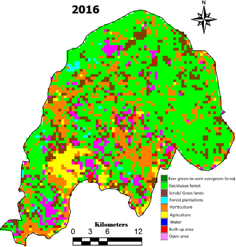
|
|
|||||||||||||||||||||||||||||||||||
| Figure 4.2.19: Status of Ramadevara Betta Vulture Sanctuary. | Table 4.2.14: Ramadevara Betta Vulture Sanctuary land use details. | |||||||||||||||||||||||||||||||||||
4.2.15 Wayanad Wild Life Sanctuary (WWLS):
Wayanad Wild Life Sanctuary form critical center for many migratory species connecting south and north portions of Western Ghats. Wayanad Wildlife Sanctuary (WWLS), a protected area in the Western Ghats have a total area of 344.44 km2. WWLS comprises of two discontinuous forest patches of 77.67 km2 (WS-I) and 266.77 km2 (WS-II). WS-II falls between 11035’N – 11049’N Latitudes & 76013’E – 76027’E Longitude and is located in the Sulthan Bathery Taluk of Wayanad District. WS-I located in Mananthavady Taluk of Wayanad District lies between the geographical extremes 11050’- 11059’N Latitude & 76002 - 7607’E Longitude. The sanctuary is administered by Wayanad Wildlife Division. WWLS was declared as a sanctuary in 1973, a part of Nilgiri Biosphere Reserve and similarly vital component for Elephant Reserve of South India. The plateau comprised of three biologically distinct regions–the main Western Ghats Mountains, the Nilgiri Hills, and the Deccan Plateau. The plateau is a contiguous network of protected areas in Karnataka (Nagarholé and Bandipur Tiger Reserve) on the eastern side and Tamilnadu (Mudumalai Tiger Reserve) on the northern side. This four protected area forms a contiguous stretch of forest having area of 2184 km2. WWLS has 45 species of mammals of which 2 species are endemic and 9 are threatened species, 227 species of birds on which 6 endemic species & 6 threatened species, 50 species of reptiles, 35 species of amphibians of which 8 are endemic species, 80 species of fishes which haves 49 endemic species & 16 threatened species) and 143 butterflies have been recorded from here The sanctuary also has the World’s largest population of Asiatic Elephants. Four-horned Antelope are also seen in this sanctuary. Red-headed and white-backed vultures, once common in Kerala are now restricted to Wayanad Plateau. Forest serves as catchments for the tributaries of Kabani River. Nagarholé-Bandipur Mudumalai-Wayanad forest patch serves as an important habitat for the tiger. Human settlements are found in Tholpetty Range, Kurichiar Range, Sulthan Bathery Range, Muthanga Range. Land use analysis and respective areas are shown in Figure 4.2.20 and Table 4.2.15. Forest constitute only 35.04 % and plantations cover 46.45 % followed by agriculture 15%. The tea estates, rubber plantations occupy major land scape region. The anthropogenic pressure is high due to many infrastructure projects and high ways.
Table 4.2.15: Wayanad Sanctuary land use details.
|
Category |
2016 |
|
|
Ha |
% |
|
|
Forest |
12080.43 |
35.04 |
|
Water Body |
597.15 |
1.73 |
|
Agriculture |
5314.47 |
15.41 |
|
Plantations |
16016.30 |
46.45 |
|
Built-Up |
157.50 |
0.46 |
|
Others |
311.31 |
0.90 |
|
Total Area |
34477.16 |
|
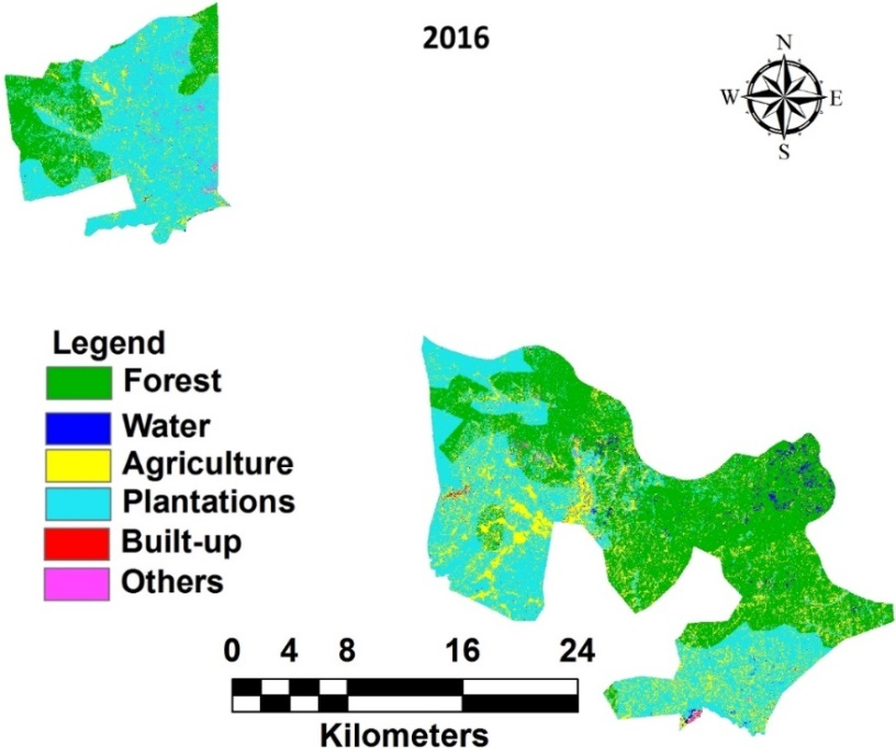
Figure 4.2.20: Land use status of Wayanad.
4.2.16 Mudumalai National Park (MNP):
Mudumalai National Park is located in northwestern side of the Nilgiri Hills in Nilgiri District of Tamil Nadu State of India. It has been declared as Tiger Reserve in the year 2007 under section 38V of the Wildlife Protection Act of 1972. The region is having rich flora and fauna diversity and also part of Nilgiri Biosphere Reserve. The forest cover is mainly tropical moist deciduous occur in the western side, where rainfall is higher than regions, tropical dry deciduous forest occurs in the middle and southern tropical dry thorn forests are in the east. MNP is contiguous with Wayanad wildlife Sanctuary on the west, Bandipur Tiger Reserve on the north, Singara Reserved Forests in the south, Satyamangalam tiger reserve (Sigur Reserved Forests) in the east. Spread over an area of 321 km² with an altitude of 1000 m and a rainfall gradient of 500 to 2000 mm. MNP plays an important role in biodiversity conservation of especially large mammals, by offering habitat contiguity of about 3300 km² with three other protected areas in the region, namely Nagarahole and Bandipur NP, MM Hills WLS and Wynaad WLS through forest corridors between the Western Ghats and Eastern Ghats has the highest potential for long-term tiger conservation, estimated tiger population of 267 (207-327) individuals occupying 9,087 km2 [10]. The flora species found in the region includes Accacia intsia, Tectona grandis, Cassia fistula, Lagestroemia microcarpa, Pterocarpus marsupium, Kydia calycina, Olea dioica, Olea glandlifera, Syzygium cumini, Erythroxylum monogynum, Mangifera indica, Pongamia glabra, Terminalia arjuna, Syzygium cumini, Dalbergia latifolia, Terminalia granulate, Ziziphus mauritiana, Albizia amara, Gnetum ula, Anogeissus latifolia and Litsea mysorensis etc. The region also has good bamboo cover supporting elephants. Larger mammals such as elephant, gaur, sambar and tiger use riparian forest patches for feeding and resting. Mammal diversity is higher in the dry deciduous and dry thorn forests than in the other habitats, 13 % of all mammal species in India present here (Ramesh et al., 2009). Tiger (Panthera tigris), leopard (Panthera pardus), and Asiatic wild dog or dhole (Cuon alpinus) are major carnivores. Chital or spotted deer (Axis axis), sambar (Rusa unicolor), muntjac or barking deer (Muntiacus muntjak), wild boar (Sus scrofa), Asian chevrotain or mouse deer (Moschiola meminna), and gaur (Bos gaurus), among the ungulates. Asian elephant (Elephas maximus), and sloth bear (Melursus ursinus) are well distributed throughout the park. Black-naped hare (Lepus nigricollis), bonnet macaque (Macaca radiate), common langur (Semnopithecus entellus), Indian porcupine (Hystrix indica), Malabar giant squirrel (Ratufa indica), and hanuman langur are other prey species.
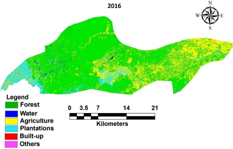
Figure 4.2.21: Status of Mudumalai NP.
MNP has 227 bird species covering 8% of bird species in India in which, 110 species are insectivores, 62 are carnivores, 23 species are fishivores, 12 species are omnivores and 20 species are granivores. These include the unique near threatened black-and-orange flycatcher, Malabar trogon, Malabar grey hornbill, Crested hawk-eagle, Crested serpent eagle, Mottled wood owl and Brown hawk owl, Golden oriole, Paradise flycatcher, Golden-backed woodpecker, Malabar great black woodpecker, Greater racket-tailed drongo etc., [11]. The construction of roads, expansion of existing state highways, other infrastructure projects are fragmenting the region in past two decades. The forest fire is other serious issue affecting the sensitive habitats. The area has invaded by Lantana camara dominated followed by Chromolaena odorata species affecting natural regeneration and grass patches. The commercial crops, inappropriate cropping pattern are resulting in wild predation of crop, leading to human-animal conflict. Land use analysis of MNP is shown in Figure 4.2.21 and Table 4.2.16. The region has 66.47 % of forest cover under various forest categories. Agriculture covers 23.96 % followed by plantations. The grazing and exotic weed infestations are disturbing major forest cover and ecology.
Table 4.2.16: MNP land use details.
|
Category |
2016 |
|
|
Ha |
% |
|
|
Forest |
25671.36 |
66.47 |
|
Water Body |
299.43 |
0.78 |
|
Agriculture |
9253.17 |
23.96 |
|
Plantations |
3296.97 |
8.54 |
|
Built-Up |
52.38 |
0.14 |
|
Others |
48.24 |
0.12 |
|
Total Area |
38621.55 |
|
4.2.17 Satyamangalam Wild Life Sanctuary (SWLS/STR):
STR is being the most important conservation unit linking western and eastern parts of Western Ghats having large carnivores and their prey population requires habitat protection along with regular monitoring. STR has been declared with an extent of 1411.609 sq.km. covering all RFs in Sathyamangalam Forest except Velamundi RF have been declared as “Sathyamangalam Wildlife Sanctuary” under section 26 A (1) (b) of Wildlife (Protection) Act 1972 with G.O. (Ms) No. 122 E&F (FR-5) Dept. dated 03.11.2008: 524.349 sq.km; G.O.(Ms) No. 93 E&F (FR-V) Dept. dated 11.08.2011: 887.260 sq.km located in Erode district. STR encompasses large contiguous Reserve Region has covered with mixed deciduous forests, tropical thorn forests and savannah types supporting numerous floral species. Flora includes Anogeissus latifolia, Santalum album, Tectona grandis, Cassia fistula, Pterocarpus marsupium, Olea dioica, Syzygium cumin, Tamarindus indica, Terminalia granulate, Ziziphus mauritiana, Albizia amara, Gnetum ula, Litsea mysorensis, Dalbergia latifolia, Mesua ferrea Hardwickia binata, Phyllanthus emblica, Mangifera indica, Pongamia glabra etc. STR is the largest Sanctuary in the state supporting major wild animals such as 64 Tigers, 924 Elephants, 3687 Wild Boars, 13442 Deers, 3189 Indian Guar. It is part of 7th Elephant Reserve (Nilgiris Eastern Ghats Elephant Reserve) and facilitates annual migration between Eastern Ghats and Western Ghats with 6 Elephant corridors. STR known for rich biodiversity has 13% of Indian mammal diversity, 225 species of birds, 30 species of reptiles, 85 species of butterflies, 15 species of amphibians, and 10 species of fishes. The area is part of India’s 1st heritage “Nilgiri Biosphere Reserve” which was declared in 1986 for its rich biodiversity and conservation value. The poaching, sandal smuggling, forest fire, encroachments are the major problems exist in STR. The land use of STR is shown in Figure 4.2.22 and Table 4.2.17 provides land use in each category. The region has 72.84 % under mixed forest cover ranging deciduous, thorny scrub, grass lands. The agriculture constitutes 17.75 % followed by plantations 9%. The anthropogenic pressure is because major villages are surrounded by forests and large amount of population are dependents on forest resources. The crop predation is high due to lack of resources in forests and attractive easy sugar based crops such as ragi, sugar cane etc.

|
|
||||||||||||||||||||||||||
| Figure 4.2.22: Status of STR. | Table 4.2.17: STR land use details. | ||||||||||||||||||||||||||
4.2.18 Chinnar Wild Life Sanctuary (CHWLS):
Chinnar Wild Life Sanctuary having a total area of 94 sq. km, located in the Eastern shadow part of Western Ghats, in Idukki district, Kerala. CWLS lies between 10° 15’ to 10° 21’ N latitude 77° 05’ to 77° 16’ E longitude. It was declared as a sanctuary in 1984. CWLS comes under Anamudi Elephant Reserve. CWLS is adjacent to Eravikulam National Park, Anamudi Shola National Park, Kurinjimala Wildlife Sanctuary in Kerala. Mostly consist of grassland, & wet grassland, some South Western Ghats montane rain forest and shola forest at high elevation. At mid elevation, dry deciduous forest and at lower elevations thorny scrub forests are seen. CWLS has the significance for its rich reptilian diversity, thorny shrub forest and also for its rich medicinal plant diversity. White bison of Manjampatti is reported from here. Grizzled Giant Squirrel, the large tree squirrel in the genus Ratufa found in the hill forests of Kerala and Tamil Nadu is the flagship species of CWLS. Sanctuary also functions as prominent catchments of an East flowing river particularly, the immediate catchment of Amaravathi reservoir in Tamil Nadu. CWLS is a harbour of flora and fauna, 34 species of mammals, 245 species of birds like Yellow Throated Bulbul, 52 species of reptiles, 42 species of fishes, 22 amphibian species and 156 butterfly species are reported. Panther, tiger, spotted deer, Indian elephants, gaur, sambar deer, common langur, tufted grey langur, bonnet macaque, hanuman langur, threatened species like Nilgiri tahr, vulnerable species like rusty spotted cats, gizzled giant squirrels etc are some of the mammalian species from this sanctuary. Of the 52 reptilian species, 29 were snakes. It also has a dwelling of Star Tortoise, Marsh Crocodile, and a large population of vulnerable Mugger Crocodiles. Chinnar and Pambar River contain Garra mullya minnows, river-carp baril, giant danio and the endangered hill stream game fish Deccan mahseer. 101 spider species have been found recently from this park. Being the part of Western Ghats make this area floristic rich. 965 species of flowering plants have been reported. Albizzia lathamii, a critically endangered tree species are found in this sanctuary. It is the only protected area in Kerala with Hill Pulaya tribal community. The land use analysis is shown in Figure 4.2.23 and Table 4.2.18. The region has good mixed forest cover of 76.35 % due to protection. The habitat types range from shola grasslands to dry thorny scrub, across a diverse cultural landscape as well. The region is also part of Anamudi elephant reserve complex supporting rich biodiversity.
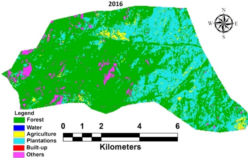
Figure 4.2.23: Status of Chinnara Sanctuary.
Table 4.2.18: CHWLS land use details.
|
Category |
2016 |
|
|
Ha |
% |
|
|
Forest |
7210.52 |
76.35 |
|
Water Body |
0.18 |
0.00 |
|
Agriculture |
113.85 |
1.21 |
|
Plantations |
1517.31 |
16.07 |
|
Built-Up |
1.62 |
0.02 |
|
Others |
600.52 |
6.36 |
|
Total Area |
9444 |
|
4.2.19 Anamudi Shola National Park (ASNP):
Anamudi Shola National Park is located in Kerala part of Western Ghats with an area covering about 42.68 sq.km. It was established as a National Park on 21st Nov 2003, one of India’s largest shola forest eco-system with a unique biodiversity and climate. The location is in between 10.160N – 10.250N Latitude and 77.150E – 77.250E, in Devikulam Taluk of Idukki District, under Munnar Wildlife Division. The park consists of three pristine shola reserve forest namely Mannavan Shola, Pullaradi shola, Idivara Shola. Mannavan Shola is the largest of them containing nearly 20% (109 species) are endemic and 25% (128species) are rare and another 26 species are threatened. The park receives high rainfall ranging between 2000-2500 mm and average temperature is between 7.5-300C. Elevation of the park is from 2152-2305 m. Strobilanthes kunthiana commenly called “Neelakurinji”, an endemic shrub is found here. It blossoms once in 12 years and when blossoms hill appears blue in color. The average height of forest is about 20-25 m which comprises of Souther subtropical hill forest; Souther montane wet temperate forest and moist deciduous forest. The park has 62 species of trees, 174 species of herbs, and shrubs 39 species of climbers are recorded. Major floral species includes Acronychia pedunculata, Ardisia rhomboidea, Cinnamomum malabaricum, Cinnamomum sulphuratum, Cryptocarya bourdillonii
Cryptocarya lawsonii, Cyathea nilgiriensis, Daphniphyllum neilgherrense, Elaeocarpus glandulosus, Elaeocarpus serratus, Gaultheria fragrantissima, Ligustrum perrottetii, Litsea floribunda, Litsea wightiana, Mahonia leschenaultia, Myrsine wightiana, Persea macrantha, Rhododendron arboretum, Strobilanthes kunthiana, Symplocos cochinchinensis, Syzygium caryophyllatum, Syzygium cumini, Syzygium densiflorum, Syzygium spathulatum, Ternstroemia japonica, Turpinia nepalensis, Vaccinium leschenaultia. Faunal distribution includes 100 species of butterflies among which Parantica nilgiriensis commonly called “Nilgiri Tiger” is one of the endemic species, 232 of moth belonging to 36 different families and 76 species of birds are recorded. Major faunal species are elephant (Elephas maximus), leopard (Panthera pardus), and Asiatic wild dog or dhole (Cuon alpinus), Chital or spotted deer (Axis axis), sambar (Rusa unicolor), muntjac or barking deer (Muntiacus muntjak), wild boar (Sus scrofa), and gaur (Bos gaurus), bonnet macaque (Macaca radiate), common langur (Semnopithecus entellus), Indian porcupine (Hystrix indica), Malabar giant squirrel (Ratufa indica), The park is protected because of the unique shola forests, its rich biodiversity and endemic and threatened species. Land use analysis (Figure 4.2.24, Table 4.2.19) highlights 62.69% of evergreen (Shola) forest cover surrounded by 31 % plantations. Crop predation by wild animals is the common problem in summer due to lack of water resources in side park. The appropriate measures are need to be considered by regulatory agencies to control the exotic and commercial plantations, which are disturbing ecology.

Figure 4.2.24: Status of Anamudi Shola.
Table 4.2.18: ASNP land use details.
|
Category |
2016 |
|
|
Ha |
% |
|
|
Forest |
2675.68 |
62.69 |
|
Water Body |
4.09 |
0.10 |
|
Agriculture |
109.98 |
2.58 |
|
Plantations |
1325.88 |
31.07 |
|
Built-Up |
0.00 |
0.00 |
|
Others |
152.37 |
3.57 |
|
Total Area |
4268 |
|
4.3. BIODIVERSITY -
FLORA AND
FAUNA DIVERSITY AND DISTRIBUTION
4.3.1 DISTRIBUTION OF FLORA SPECIES:
The Cauvery river basin is rich in flora diversity and rightfully enough to constitute a separate phyto-geographic unit. The flora distribution has shown in Figure 4.3.1 implies there are 486 variety of species present in the basin as per literatures. The database consists 2200 entries of various flora species and Annexure 1 provides detailed description such as species name, family name, local names, uses, etc. The major floral species are having higher medicinal values, anti-microbial properties and socio-economically significant. The flora species (486) belong to 116 families across the basin. The Lauraceae, Fabaceae, Myrtaceae, Poaceae, Rubiaceae are the dominant families found in the basin. The region has highly endemic species around (147 species) such as Artocarpus hirsutus, Atalantia wightii, Blachia umbellate, Cinnamomum macrocarpum, Cinnamomum malabaricum, Cinnamomum travancoricum, Diospyrous paniculata, Garcinia gummi-gutta, Holigarna grahamii, Hopea ponga, Ixora brachiata, Knema attenuate, Pinanga dicksonii, Syzygium densiflorum, Syzygium malabaricum, Terminalia travancorensis, Vateria indica etc. Increase in the anthropogenic pressures within the river basin and surrounding landscapes have persistently stressed the ecosystem structure adversely, besides altering its composition. Figure 4.3.2 outlines the distribution of flora species as per IUCN categories (CR-critically endangered, EN-endangered VU-vulnerable, DD-data deficient, LC-least concerned, NT-near threatened, DD- data deficient, EX-extinct, NE-not evaluated).
The CR category represents (Figure 4.3.3) Cinnamomum travancoricum, Memecylon sisparense, Vateria indica and Vateria macrocarpa species which are confined to major portions of Southern Western Ghats partly seen in central Western Ghats. The Figure 4.3.4 represents EN category consisting major species of Actinodaphne salicina, Beilschmiedia wightii, Cinnamomum wightii, Dysoxylum malabaricum, Hopea parviflora, Hopea ponga, Syzygium caryophyllatum, and Xylosma latifolium. The species shown in VU, EN, CR are the belongs to primary forest vegetation types implies the need for more protection. The region is suffering from unethical encroachments, land use changes, unplanned infrastructure developments and increase in human population etc. Sunil et al., 2010 highlights how vegetation density and site disturbance scores of various streams reveals that mining and grazing areas in the catchment have exerted negative impact on riparian forest. Figure 4.3.5 represents species of VU category includes Actinodaphne malabarica, Artocarpus hirsutus, Calophyllum apetalum, Canthium dicoccum, Cinnamomum agasthyamalayanum, Cinnamomum macrocarpum, Cinnamomum malabaricum, Michelia nilagirica, Syzygium densiflorum and Tarenna nilagirica etc. Figure 4.3.6 represents species of NT category includes Elaeocarpus munronii, Goniothalamus wynaadensis, Gordonia obtuse, Heritiera papilio, Holigarna grahamii, Litsea mysorensis and Sageraea laurifolia. Figure’s 4.3.7, 4.3.8 and 4.3.9 represent categories of LC, DD, NE covering 440 species.
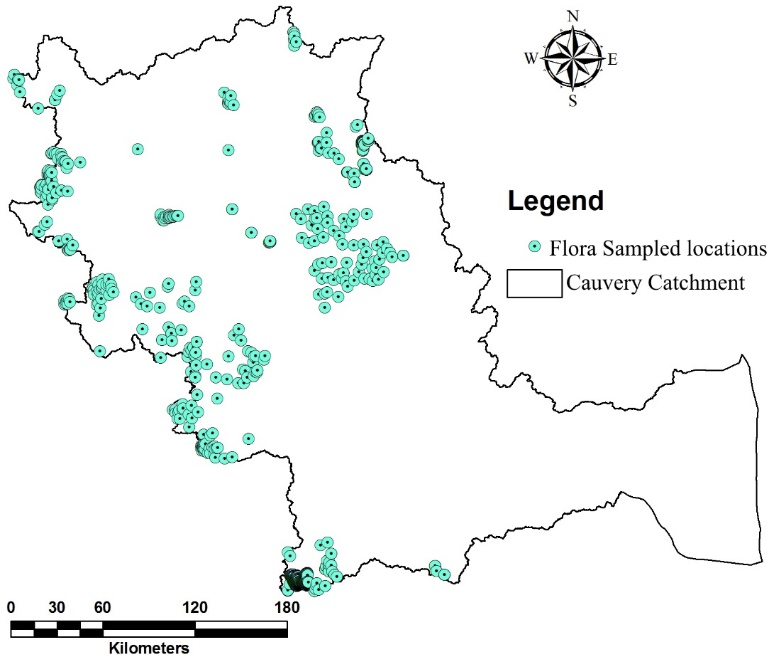
Figure 4.3.1: Flora sampled locations.

Figure 4.3.2: Distribution of Flora as per IUCN categories.
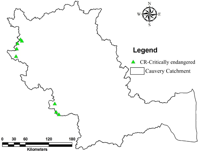
Figure 4.3.3: Distribution of Flora as per IUCN-CR category.
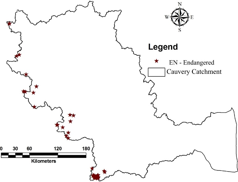
Figure 4.3.4: Distribution of Flora as per IUCN-EN category.
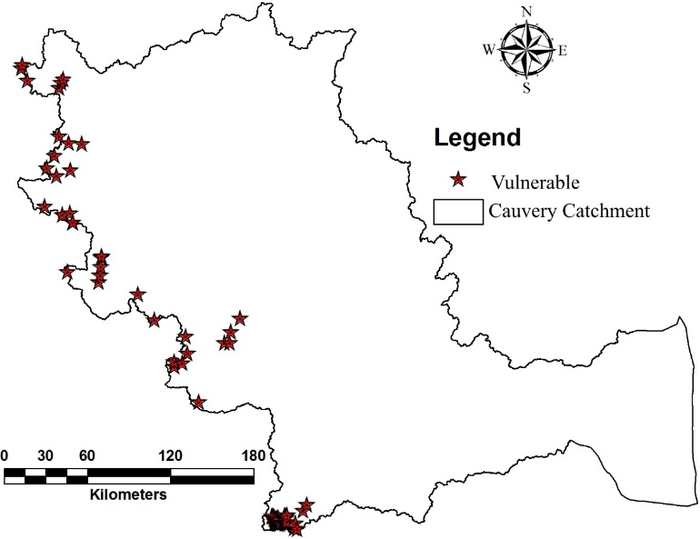
Figure 4.3.5: Distribution of Flora as per IUCN-VU category.
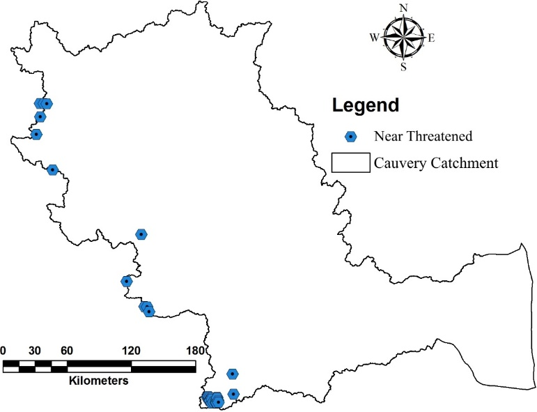
Figure 4.3.6: Distribution of Flora as per IUCN-NT category.
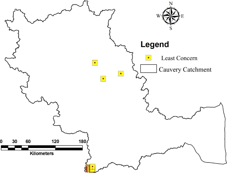
Figure 4.3.7: Distribution of Flora as per IUCN-LC category.
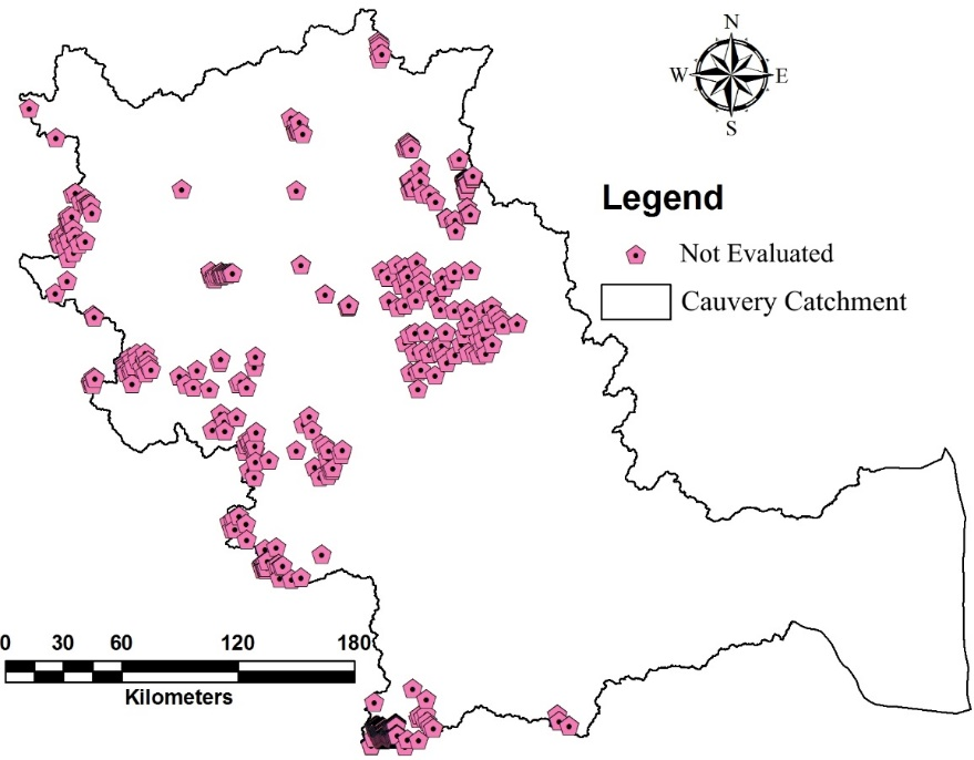
Figure 4.3.8: Distribution of Flora as per IUCN-NE category.

Figure 4.3.9: Distribution of Flora as per IUCN-DD category.
4.3.2 DISTRIBUTION OF FAUNAL SPECIES:
The review covered articles from national and international journals and forest action plans. As per the mined data, Cauvery basin has total 771 species under 183 families (Table 4.3.1) in which, 42 species of fishes under 11 families, 10 species of crabs under 6 families, 74 species of amphibians under 10 families, 80 species of reptiles under 19 families, 388 bird species under 88 families, 51 butterflies under 9 families, 27 insects under 9 families, and 99 mammalian species under 31 families. The review has around 3033 entries of various faunal species (Figure 4.3.10) covering Amphibians, Mammals, Fishes, Birds, Insects, Butterflies, details are provided in Annexure 2. The data base contains details such as Sno, Latitude, Longitude, Species Name, Location, Source, Common Name, Type, Family Name, IWPA (Indian Wildlife Protection Act), IUCN Status, Remarks and Endemism. Cauvery basin is the abode for many endemic critically endangered species, emphasizing its ecological sensitivity. Amphibians show higher endemism followed by reptiles, mammals, fishes and birds. The literature also revealed that many numbers of threatened and endemic species are present across 253 sampled locations (Figure 4.3.11). Cauvery region is one of unique region of biological and ecological importance and is irreplaceable if destroyed. Serving as a prime habitat for several species of amphibians, reptiles, birds and mammals comprising Tiger (Panthera tigris), Asian Elephant (Elephas maximus), Indian gaur (Bos gaurus), Sambar deer (Cervus unicolor), Spotted deer (Axis axis), Leopard (Panthera pardus), Wild dog (Cuon alpines), Sloth bear (Melurus ursinus), Smooth coated otter (Lutrogale perspicillata), Pangolin (Manis crassicaudata), Slender loris (Loris lardigradus) and Black naped hare (Lepus nigricollis), etc.
Table 4.3.1: list of faunal species and their details
|
Sl.no |
Faunal Type |
Number of Species |
Number of Families |
|
1 |
Fish |
42 |
11 |
|
2 |
Crabs |
10 |
6 |
|
3 |
Amphibians |
74 |
10 |
|
4 |
Reptiles |
80 |
19 |
|
5 |
Insects |
27 |
9 |
|
6 |
Butterflies |
51 |
9 |
|
7 |
Birds |
388 |
88 |
|
8 |
Mammals |
99 |
31 |
|
Total |
771 |
183 |
|
As per IUCN red list categories the major basin covers various species of importance as shown in Figure 4.3.12. IUCN CR category represent species of Barbodes wynaadensis, Campephilus imperialis, Gyps bengalensis, Gyps indicus, Hemibagrus punctatus, Indirana gundia, Mystus punctatus, Petinomys fuscocapillus, Philautus ponmudi, Puntius wynaadensis, Sarcogyps calvus and Viverria civettinaas etc. as shown in Figure 4.3.13. IUCN EN category represent species of Cnemaspis wynadensis, Colias nilagiriensis, Cuon alpinus, Elephas maximus, Eumyias albicaudata, Ghatixalus variabilis, Latidens salimalii, Loris tardigradus, Manis crassicaudata, Neophron percnopterus, Panthera tigris, Philautus charius, Philautus wynaadensis and Tor khudree etc. as shown in Figure 4.3.14. The region has VU category species such as Anthus nilghiriensis, Bos gaurus, Cervus unicolor, Cnemaspis indica, Indotestudo travancoria, Martes gwatkinsii, Melursus ursinus, Montecincla fairbanki, Nyctibatrachus major, Panthera pardus, Philautus dubois, Rusa unicolor, Tetracerus quadricornis and Trachypithecus johnii suffering higher anthropogenic pressure across basin (Figure 4.3.15). The TN category reflects the threatened species of the basin such as Anhinga melanogaster, Antilope cervicapra, Chloropsis cochinchinensis, Eumyias albicaudatus, Ficedula nigrorufa, Hyaena hyaena, Mycteria leucocephala, Parantica nilgiriensis, Phylloscopus tytleri, Psittacula roseate, Pycnonotus priocephalus, Python molurus, Sterna aurantia, Threskiornis melanocephalus, and Wallago attu etc., as shown in Figure 4.3.16. The region has some of the extent species (EX) such as White_nosed Bush Frog (Philautus leucorhinus) and Plain Coloured Bush Frog (Philautus temporalis) as shown in Figure 4.3.17. The region represents 423 faunal species across various locations under LC category as shown in Figure 4.3.18. There are around 210 species represent under NE category as shown in Figure 4.3.19, emphasizes lack of detailed studies to understand threat status. The region is suffering high human animal conflict, loss of faunal diversity due to population pressure, encroachment of forests, forest fires, fragmentation, poaching etc.
Fish as food has been harvested for several decades but during the past 3-4 decades the exploitations have been on an intensive scale resulting in diminished populations in the basin. The major fish population present in the basin fall under CR, EN categories reflecting the threat faced by taxa. Continuous discharge of industrial wastes, residues and untreated sewage entering from town, cities have adversely affected fish growth and population. Siltation, mining activities, land use activities harmful fishing practices such as poisoning and dynamiting fish etc. are adversely impacting habitat and causing the decline of indigenous fish and fisheries resources. Constructions of dams, weirs and barrages have resulted in stagnant water bodies and confined fish habitats. The introduced fishes to meet the growing demand, laid more stress on the culture of fast‐growing Indian major carps Catla catla, Labeo rohita and Cirrhinus mrigala. These introduced fish species have adopted well in freshwater. Since few years, the introduced Cyprinus carpio (Common carp) and inadvertently entered Oreochromis mossambica (Tilapia) have dominated in the inland water fishery, as they breed and multiply fast in a short span of time.
The Cauvery basin serves as a major habitat for elephants across three states such as Karnataka, Tamil Nadu, Kerala. The basin has large population distributed across there states and they migrate from one place to other for food and other purposes. They follow defined path well known as Mysore elephant reserve zone as shown in Figure 4.3.20. The elephants move from Pushpagiri Wild Life Sanctuary (PWLS) located in northern top portion of basin to Southern eastern portion of Tamil Nadu state (Satya Mangalam forest, Tali reserve forest etc.,) (Figure 4.3.21). Figure 4.3.22 depicts forest cover as per 1965 vegetation map of South India, represent major portion had dense forest cover. With increase in anthropogenic activities, region has lost major forest cover depicted by land use map of 2017 (Figure 4.3.23, 4.3.24). Region has been replaced with horticulture activities, exotic plantations, commercial crops and other land uses at the cost of native forests. The major portion of migratory path is highly disturbed with human activities leading to human-animal conflict. Fragmentation of forests in the region has impacted the habitat of wild fauna, evident from frequent human-animal conflicts, crop predation by elephants, etc. The electrocuting an elephant, illicitly taping live electric connection to fences, hunting or shooting is the common practice of farmers to protect crops. The incident of killing of wild animals by man as a retaliation against physical attack and against crop depredation has taken a toll of considerable number of wild animals around the park. The fragmentation and blocking of elephant migratory paths have impacted the movement of wild animals.
Cauvery basin can be considered as an ecological hotspot of diversity due to presence of endemic flora and faunal species supporting various life forms. Figure 4.3.25 shows flora, fauna distribution studied, highlights central portion has major diversity due to forest cover of Western Ghats Eastern Ghats and reserve forests. Figure 4.3.26 highlights species distribution and portrays current land use. The abrupt changes can be noticed as compared with 1965 vegetation map due to senseless developmental thrust and market based agro-economic activities. The native forests are replaced with exotic plantations, encroachment, horticulture crops resulting in loss of diversity.
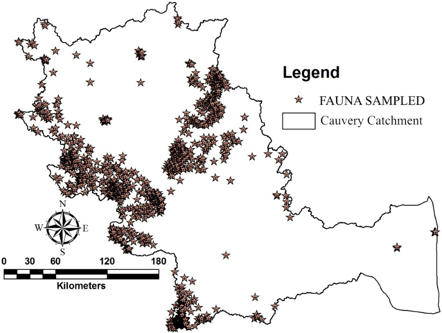
Figure 4.3.10: Faunal distribution based on type.
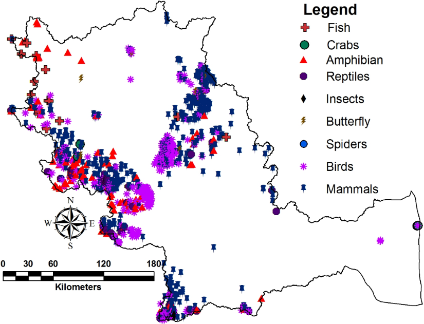
Figure 4.3.11: Fauna distribution and sampled locations.
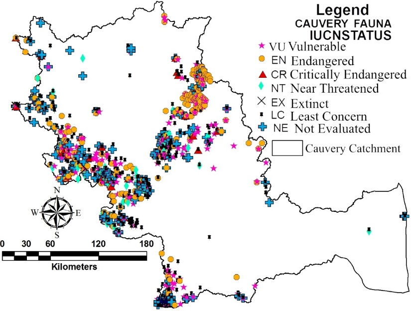
Figure 4.3.12: Fauna distribution as per IUCN status.

Figure 4.3.13: Distribution as per IUCN- CR status.
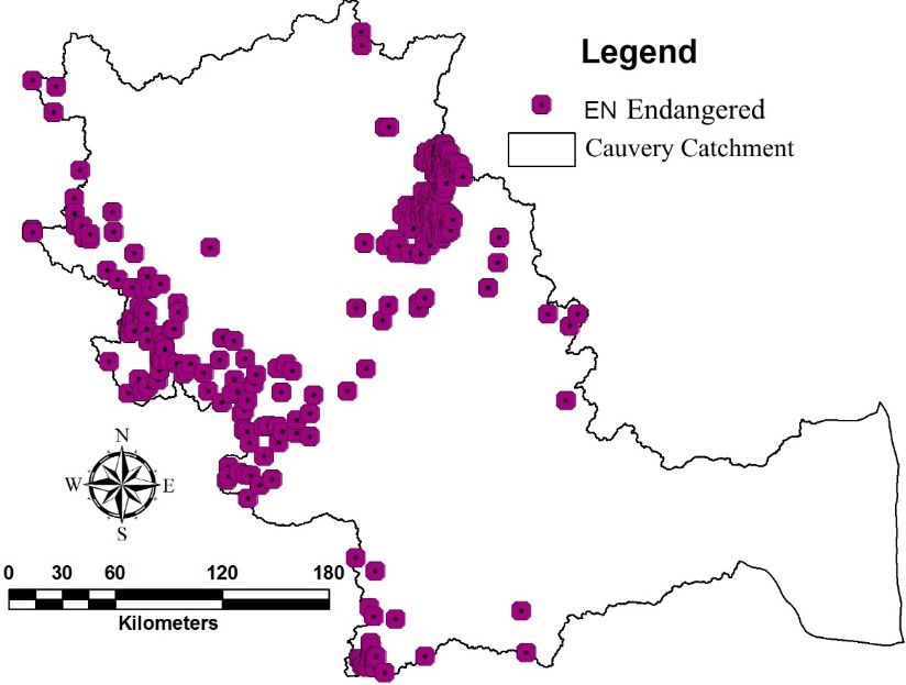
Figure 4.3.14: Distribution as per IUCN- EN status.
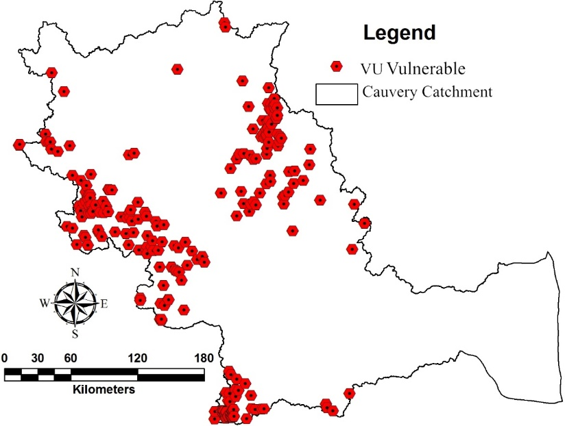
Figure 4.3.15: Distribution as per IUCN- VU status.

Figure 4.3.16: Distribution as per IUCN- NT status.

Figure 4.3.17: Distribution as per IUCN- EX status.
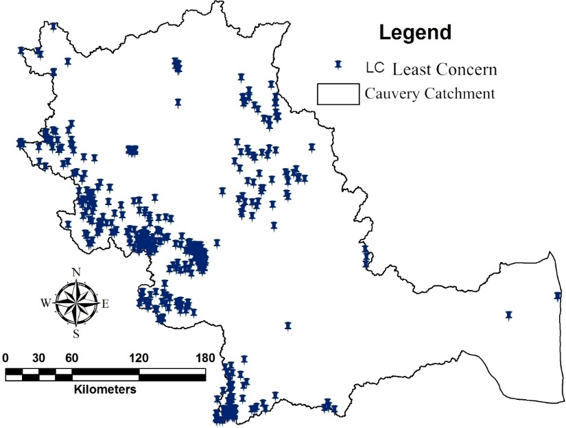
Figure 4.3.18: Distribution as per IUCN- LC status.
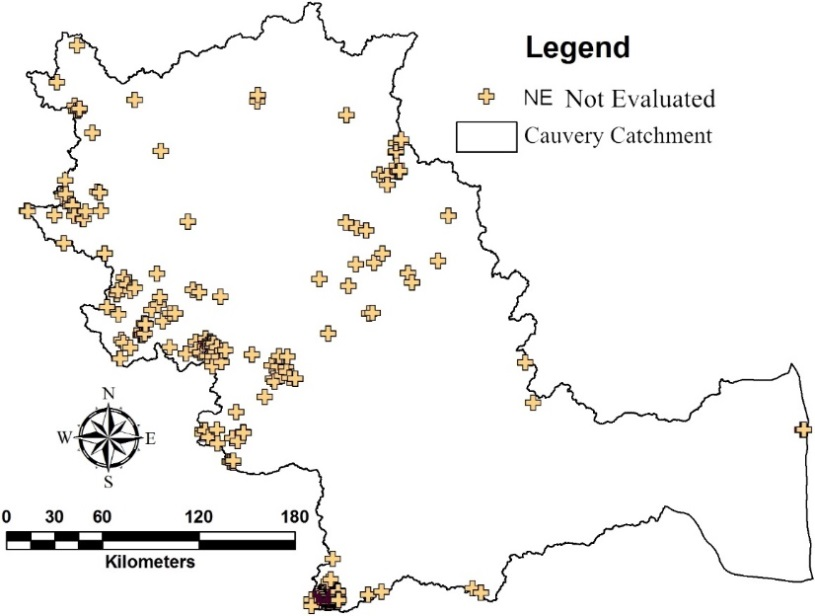
Figure 4.3.19: Distribution as per IUCN- NE status.

Figure 4.3.20: Elephant movement path of in Cauvery basin (Mysore Elephant Reserve).

Figure 4.3.21: Elephant movement path (EMP) from Pushpagiri WLS (Karnataka
State)
to Satyamangalam Forest (Tamil Nadu State).

Figure 4.3.22: Forest cover in EMP as per 1965 vegetation map.
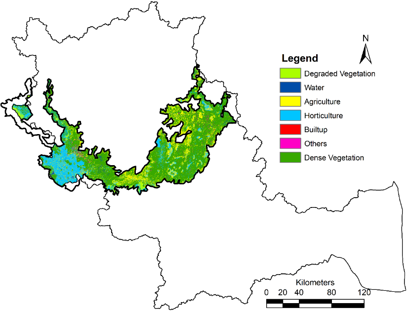
Figure 4.3.23: Status of EMP asper land use map 2017.
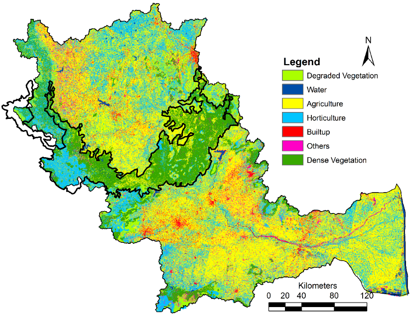
Figure 4.3.24: Cauvery land use map and EMP.

Figure 4.3.24: Cauvery basin- flora & fauna.

Figure 4.3.25: Cauvery basin land use map (2017) and distribution of flora, fauna.
4.4. HYDROLOGY
RAINFALL: In order to extract the rainfall data from GPCC at each agro climatic zone, Girds were created and point sampling tool was used to extract spatiotemporal data on rainfall. Figure 4.4.1 depicts point grid map that was used to extract precipitation information.
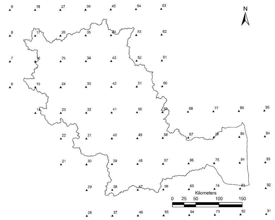
Figure 4.4.1: Point Grids in and around Cauvery river basin
Based on the agro climatic map and administrative boundaries, about 77 point grids were classified as i) Kerala portion of Western Ghats, ii) Karnataka portion of Western Ghats, iii) Tamil Nadu portion of Western Ghats, iv) Deccan Plateau of Karnataka, v) Eastern Ghats and Uplands of Tamil Nadu and vi) East Coast of Tamil Nadu.
Kerala portion of Western Ghats: Average annual rainfall in the Western Ghats part of Kerala varies between 2700 mm to over 3500 mm across space, Figure 4.4.2 to 4.4.4 and Table 4.4.1 depicts the Rainfall dynamics and characteristics of one of the point grid station (Grid point id 22). The Trend line shows gradually decreasing pattern of rainfall. Average rainfall in the station is about 3315 mm with lowest of 2436 and highest of 5872 mm, Standard deviation about 531 mm with COV of 0.16. Rainfall dependability at 90% is 3150 mm, at 75% is 3390 mm and at 50% is 3720 mm, the average rainfall of 3315 mm has a dependability about 78.7%. Based on the IMD classification normal rainfall in the station (id 22) varies between 2652 mm to 3979 mm which has the probability of occurrence of 0.81with rainfall return period of 1.2 year.
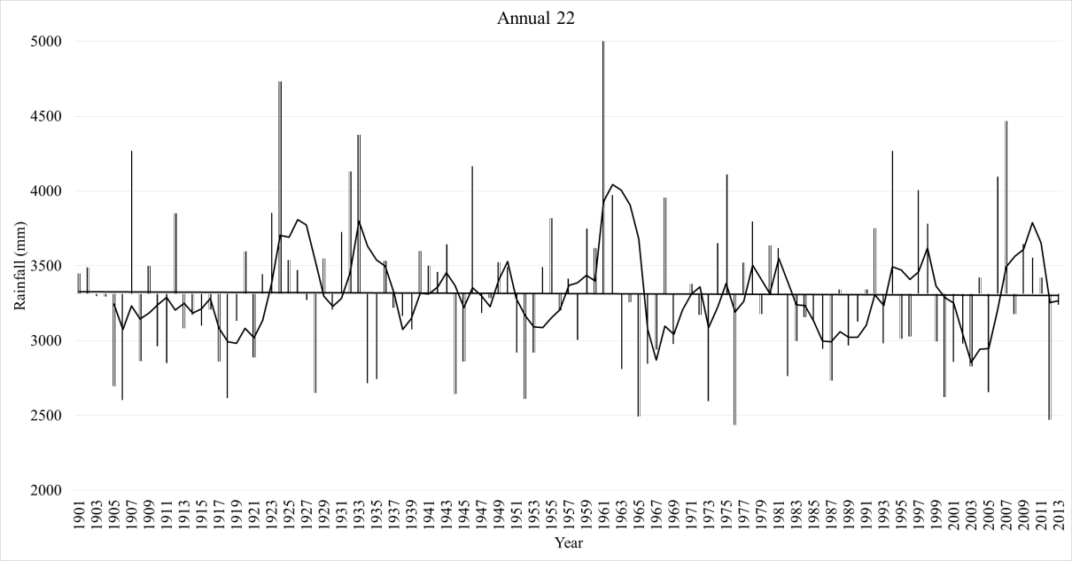
Figure 4.4.2: Rainfall trend in Kerala– Western Ghats
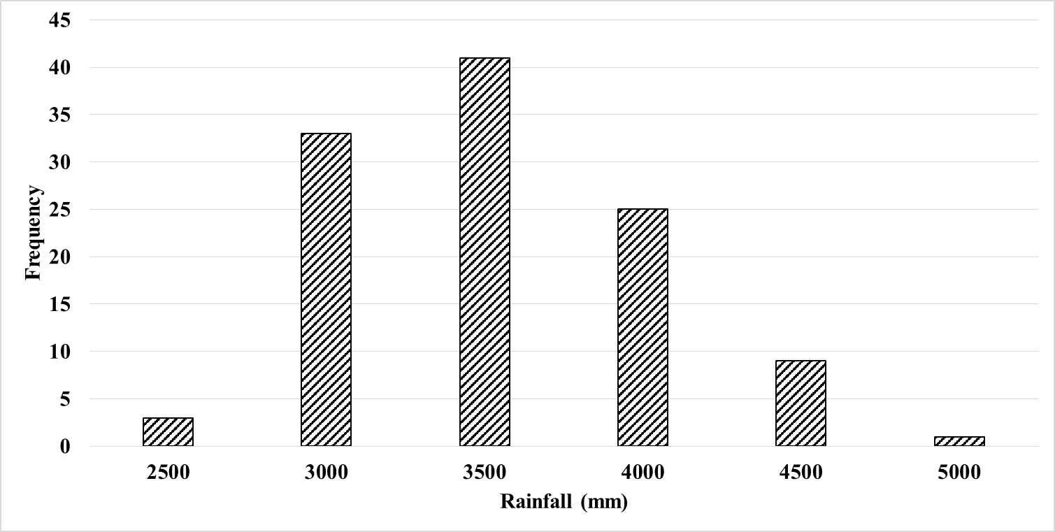
Figure 4.4.3 : Rainfall frequency in Kerala– Western Ghats
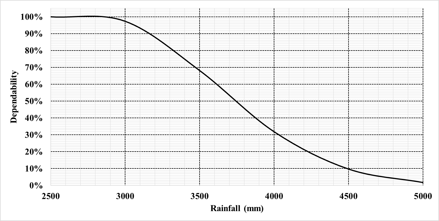
Figure 4.4.4: Rainfall Dependability in Kerala– Western Ghats
Table 4.4.1: Rainfall Characteristics of Cauvery in Kerala– Western Ghats
|
Rainfall (mm) |
Frequency |
Probability of Occurrence |
Dependability |
Return Period (years) |
|||||||
|
2500 |
3 |
0.03 |
100% |
37.7 |
|||||||
|
3000 |
33 |
0.29 |
97% |
3.4 |
|||||||
|
3500 |
41 |
0.36 |
68% |
2.8 |
|||||||
|
4000 |
25 |
0.22 |
32% |
4.5 |
|||||||
|
4500 |
9 |
0.08 |
10% |
12.6 |
|||||||
|
5000 |
1 |
0.01 |
2% |
113.0 |
|||||||
|
Minimum |
2436mm |
Maximum |
5872mm |
||||||||
|
Mean |
3315mm |
Median |
3067mm |
||||||||
|
Standard Deviation |
± 531.93mm |
Coefficient of Variation |
0.16 |
||||||||
|
Dependability |
90% |
75% |
50% |
||||||||
|
Rainfall (mm) |
3150 |
3390 |
3720 |
||||||||
|
Indian Meteorological Department – Rainfall Distribution All India Scenario |
|||||||||||
|
Rainfall |
Condition |
Rainfall |
Probability
of |
Return
Period |
|||||||
|
Severe Drought |
> -60% Average |
<1989 |
0.00 |
- |
|||||||
|
Drought |
-60% Average to - 20% Average |
1989-2652 |
0.09 |
11.3 |
|||||||
|
Normal |
± 20% Average |
2652-3979 |
0.81 |
1.2 |
|||||||
|
Excess |
> 20% Average |
>5872 |
0.10 |
10.3 |
|||||||
Karnataka portion of Western Ghats: Similar to Kerala, Karnataka portion of Western Ghats receives average annual rainfall between 2500 to 5000 mm. Figure 4.4.5 to 4.4.7 and Table 4.4.2 depicts the Rainfall dynamics and characteristics of one of the point grid station (Grid point id 15). Rainfall trend shows a decreasing pattern across the time period with average rainfall of 4196 mm with minimum and maximum being 3162mm and 6189 mm respectively. Normal rainfall as per the IMD has a return period of 1.13 years with probability of occurrence of 0.88.

Figure 4.4.5: Rainfall Trend in Karnataka– Western Ghats
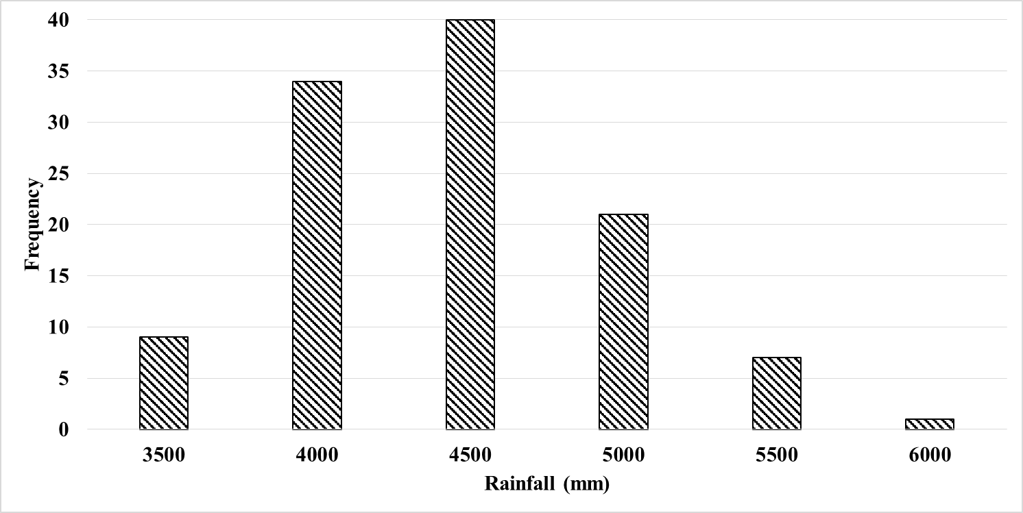
Figure 4.4.6: Rainfall frequency in Karnataka– Western Ghats

Figure 4.4.7: Rainfall dependability in Karnataka– Western Ghats
Table 4.4.2: Rainfall Characteristics of Cauvery in Karnataka – Western Ghats
|
Rainfall (mm) |
Frequency |
Probability of Occurrence |
Dependability |
Return Period (years) |
|||||||
|
3500 |
9 |
0.08 |
100% |
12.6 |
|||||||
|
4000 |
34 |
0.30 |
92% |
3.3 |
|||||||
|
4500 |
40 |
0.35 |
62% |
2.8 |
|||||||
|
5000 |
21 |
0.19 |
27% |
5.4 |
|||||||
|
5500 |
7 |
0.06 |
8% |
16.1 |
|||||||
|
6000 |
1 |
0.01 |
2% |
113.0 |
|||||||
|
Minimum |
3162mm |
Maximum |
6589mm |
||||||||
|
Mean |
4196mm |
Median |
3938mm |
||||||||
|
Standard Deviation |
± 556.98mm |
Coefficient of Variation |
0.13 |
||||||||
|
Dependability |
90% |
75% |
50% |
||||||||
|
Rainfall (mm) |
4050 |
4300 |
4660 |
||||||||
|
Indian Meteorological Department – Rainfall Distribution All India Scenario |
|||||||||||
|
Rainfall |
Condition |
Rainfall |
Probability
of |
Return
Period |
|||||||
|
Severe Drought |
> -60% Average |
< 2518 |
0 |
- |
|||||||
|
Drought |
-60% Average to - 20% Average |
2518 - 3357 |
0.044 |
22.6 |
|||||||
|
Normal |
± 20% Average |
3357 - 5035 |
0.88 |
1.13 |
|||||||
|
Excess |
> 20% Average |
> 6589 |
0.071 |
14.12 |
|||||||
Karnataka portion of Deccan Plateau: This portion one of the driest belt with average rainfall varying between 480 mm to nearly 1700 mm at the transition zone between the Ghats and plateau with COV varying upto 0.33. Figures 4.4.8 to 4.4.10 and Table 4.4.3 depict the rainfall pattern at one of the point grid station (id: 53). The trend line doesn’t show much of a variability across time. The average rainfall in the station is about 697 mm with minimum and maximum rainfall observations of 368 and 1264 mm. Normal rainfall at the station ranges between 558mm to 836 mm with probability of occurrence of 0.58 and return period of 1.7 years, drought and excess rainfall conditions prevail with probability of 0.19 and 0.17 with return period of 5.1 and 5.7 years respectively.

Figure 4.4.8: Rainfall Trend in Karnataka– Deccan Plateau
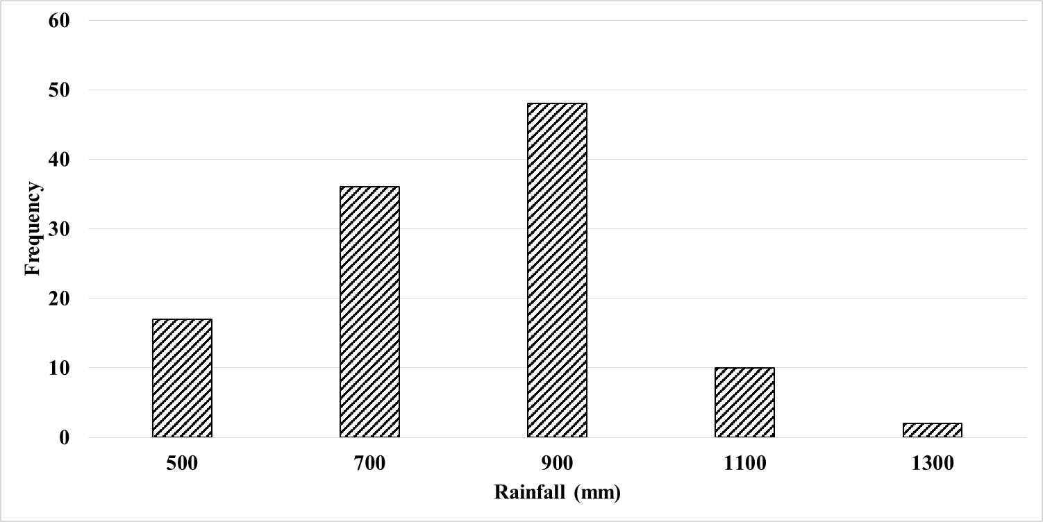
Figure 4.4.9: Rainfall frequency in Karnataka – Deccan Plateau
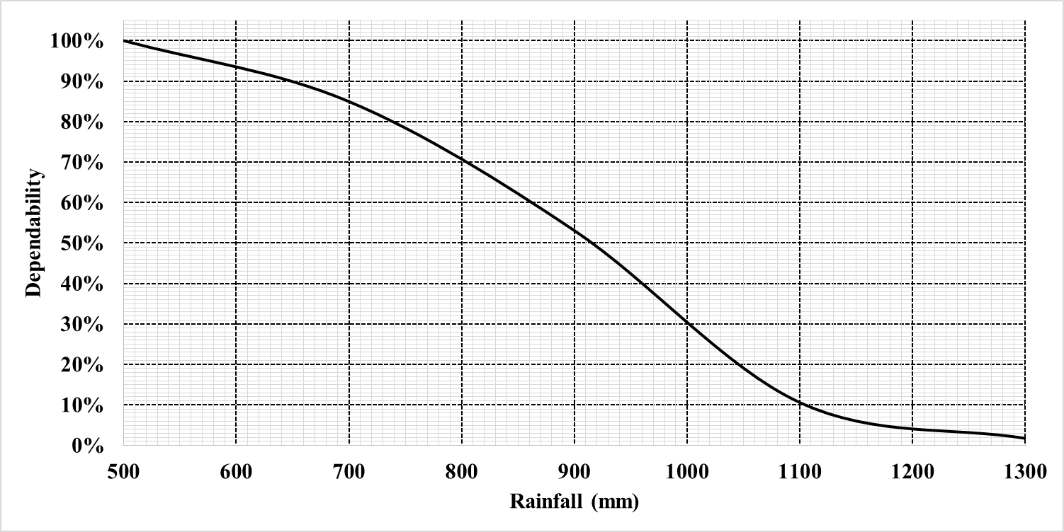
Figure 4.4.10: Rainfall dependability in Karnataka – Deccan Plateau
Table 4.4.3: Rainfall Characteristics of Cauvery in Karnataka – Deccan Plateau
|
Rainfall (mm) |
Frequency |
Probability of Occurrence |
Dependability |
Return Period (years) |
|||||||
|
500 |
17 |
0.15 |
100% |
6.6 |
|||||||
|
700 |
36 |
0.32 |
85% |
3.1 |
|||||||
|
900 |
48 |
0.42 |
53% |
2.4 |
|||||||
|
1100 |
10 |
0.09 |
11% |
11.3 |
|||||||
|
1300 |
2 |
0.02 |
2% |
56.5 |
|||||||
|
Minimum |
368mm |
Maximum |
1264mm |
||||||||
|
Mean |
697mm |
Median |
600mm |
||||||||
|
Standard Deviation |
± 173.44mm |
Coefficient of Variation |
0.25 |
||||||||
|
Dependability |
90% |
75% |
50% |
||||||||
|
Rainfall (mm) |
650 |
770 |
940 |
||||||||
|
Indian Meteorological Department – Rainfall Distribution All India Scenario |
|||||||||||
|
Rainfall |
Condition |
Rainfall |
Probability
of |
Return
Period |
|||||||
|
Severe Drought |
> -60% Average |
<418 |
0.044 |
22.6 |
|||||||
|
Drought |
-60% Average to - 20% Average |
418 -558 |
0.195 |
5.1 |
|||||||
|
Normal |
± 20% Average |
558 -836 |
0.584 |
1.7 |
|||||||
|
Excess |
> 20% Average |
>1265 |
0.177 |
5.7 |
|||||||
Eastern Ghats and Uplands of Tamil Nadu: Tamil Nadu inlands areas also one of the driest belt next to Karnataka portion of Deccan Plateau in Cauvery basin. This region has an average annual rainfall ranging between 640mm to 1750 mm at transition zones with coefficient of variation up to 0.22. Figures 4.4.11 to 4.4.13 and Table 4.4.4 depict the rainfall pattern in one of the grid (id: 57) in the plateau of Tamil Nadu. The trend line doesn’t show variability across time. Average rainfall in the station is about 641 mm with minimum and maximum observations of 346 mm and 1024 mm respectively. Normal rainfall ranges between 513 mm and 770 mm with probability of occurrence of 0.64 and return period of 1.6 years, both drought and excess cases occur at a probability of 0.17 with return period of 5.9 years.
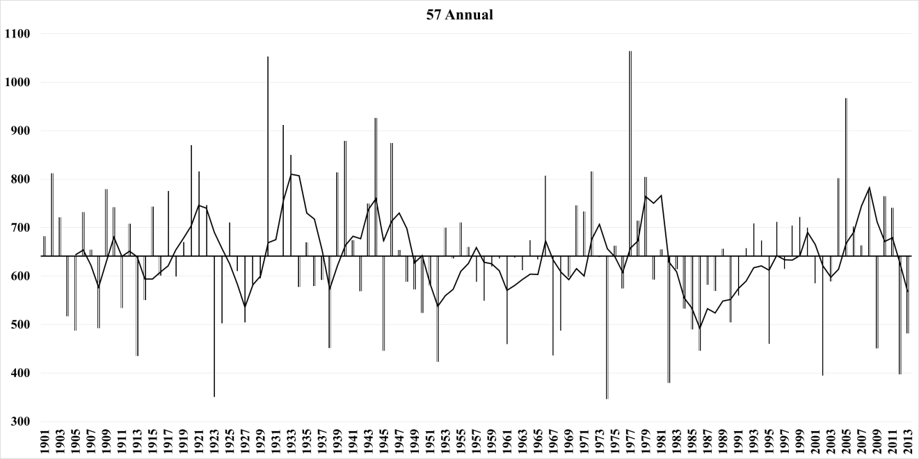
Figure 4.4.11: Rainfall trend in Tamil Nadu– Uplands

Figure 4.4.12: Rainfall frequency in Tamil Nadu-Uplands

Figure 4.4.13: Rainfall dependability in Tamil Nadu-Uplands
Table 4.4.4: Rainfall Characteristics of Cauvery in Tamil Nadu – Uplands
|
Rainfall (mm) |
Frequency |
Probability of Occurrence |
Dependability |
Return Period (years) |
|||||||
|
500 |
19 |
0.17 |
100% |
5.9 |
|||||||
|
700 |
56 |
0.50 |
83% |
2.0 |
|||||||
|
900 |
33 |
0.29 |
34% |
3.4 |
|||||||
|
1100 |
5 |
0.04 |
4% |
22.6 |
|||||||
|
Minimum |
346mm |
Maximum |
1064mm |
||||||||
|
Mean |
641mm |
Median |
522mm |
||||||||
|
Standard Deviation |
± 141.93mm |
Coefficient of Variation |
0.22 |
||||||||
|
Dependability |
90% |
75% |
50% |
||||||||
|
Rainfall (mm) |
640 |
740 |
830 |
||||||||
|
Indian Meteorological Department – Rainfall Distribution All India Scenario |
|||||||||||
|
Rainfall |
Condition |
Rainfall |
Probability
of |
Return
Period |
|||||||
|
Severe Drought |
> -60% Average |
<385 |
0.03 |
37.7 |
|||||||
|
Drought |
-60% Average to - 20% Average |
385-513 |
0.17 |
5.9 |
|||||||
|
Normal |
± 20% Average |
513-770 |
0.64 |
1.6 |
|||||||
|
Excess |
> 20% Average |
>1065 |
0.17 |
5.9 |
|||||||
East Coastal portion of Tamil Nadu: East Coast of Tamil Nadu receives rain average annual rainfall between 845 mm to 1300 mm, with coefficient of variation ranging up to 0.24. Figures 4.4.14 to 4.4.16 and table 4.4.5 depicts the rainfall patterns, and characteristics of an east coast station (id: 84). Trend line shows no variability across time. Average rainfall in the station is about 1034 mm with minimum and maximum rainfall ranging between 815 mm and 1832 mm respectively. Normal rainfall ranges between 813mm and1240 mm with occurrence probability of 0.59 and return period of 1.6 years, Droughts are prone to occur with return period of 5.3 year and excess with return period of 4.7 years
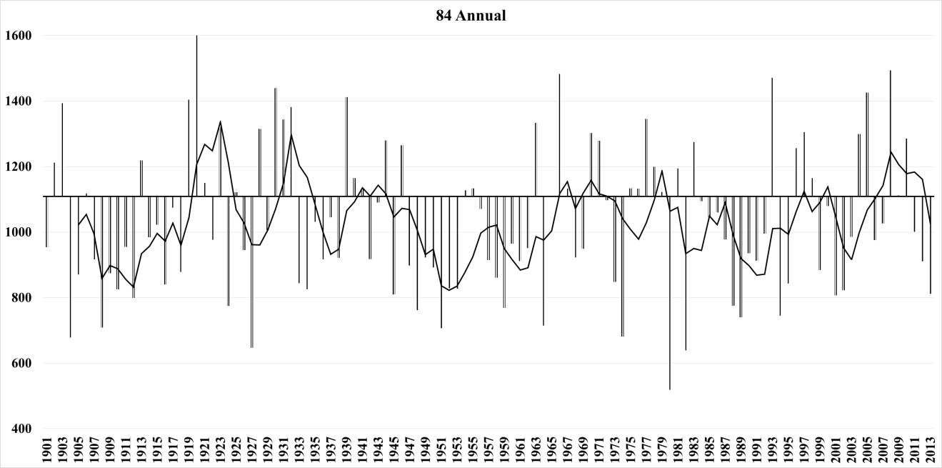
Figure 4.4.14: Rainfall trend in Tamil Nadu– East Coast
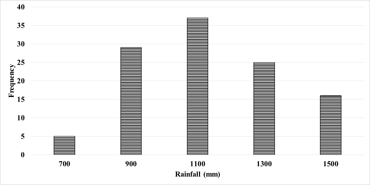
Figure 4.4.15: Rainfall frequency in Tamil Nadu– East Coast
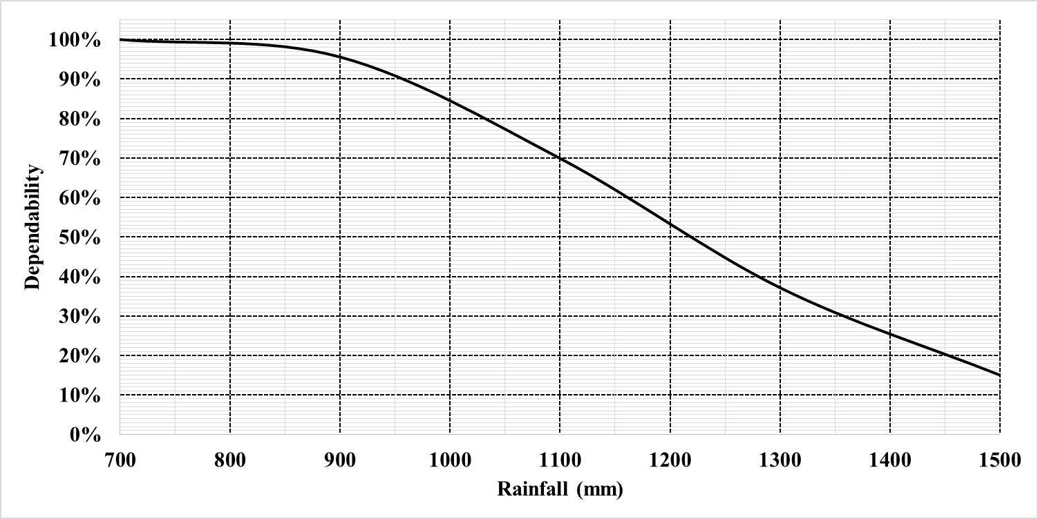
Figure 4.4.16: Rainfall dependability in Tamil Nadu– East Coast
Table 4.4.5: Rainfall Characteristics of Cauvery in Tamil Nadu – East Coast
|
Rainfall (mm) |
Frequency |
Probability of Occurrence |
Dependability |
Return Period (years) |
|||||||
|
700 |
5 |
0.04 |
100% |
22.6 |
|||||||
|
900 |
29 |
0.26 |
96% |
3.9 |
|||||||
|
1100 |
37 |
0.33 |
70% |
3.1 |
|||||||
|
1300 |
25 |
0.22 |
37% |
4.5 |
|||||||
|
1500 |
16 |
0.14 |
15% |
7.1 |
|||||||
|
Minimum |
815mm |
Maximum |
1832mm |
||||||||
|
Mean |
1034mm |
Median |
853mm |
||||||||
|
Standard Deviation |
± 229.41mm |
Coefficient of Variation |
0.22 |
||||||||
|
Dependability |
90% |
75% |
50% |
||||||||
|
Rainfall (mm) |
950 |
1160 |
1220 |
||||||||
|
Indian Meteorological Department – Rainfall Distribution All India Scenario |
|||||||||||
|
Rainfall |
Condition |
Rainfall |
Probability
of |
Return
Period |
|||||||
|
Severe Drought |
> -60% Average |
<620 |
0.009 |
113 |
|||||||
|
Drought |
-60% Average to - 20% Average |
610 -827 |
0.186 |
5.3 |
|||||||
|
Normal |
± 20% Average |
813-1240 |
0.593 |
1.687 |
|||||||
|
Excess |
> 20% Average |
>1832 |
0.212 |
4.7 |
|||||||
Note: Statistical analysis of rainfall, graphical represnetations for all 77 stations are presented in annexure 3.
In order to understand rainfall patterns across space in a detailed manner, higher resolution data of 1 kilometer resolution from WorldClim [12] was used. Figure 4.4.17 depicts monthly rainfall dynamics within Cauvery catchment. Catchment receives rainfall across two rainy seasons i.e., South West Monsoon and North East Monsoons between June to December and with local rains during April and May months. Karnataka, Kerala and Western Ghats of Tamil Nadu is dominated by south west monsoons, whereas Coastal and Interior Tamil Nadu is dominated by North east monsoons. Cauvery basin on an average receives annual rainfall of 957 mm where in the South West monsoons contribute to 362 mm of Rainfall and North East contributes to 237 mm of rainfall. Table 4.4.6 depicts the rainfall dynamics across seasons
Table 4.4.6: Rainfall dynamics across seasons and administrative divisions
|
Rainfall |
units |
Kerala |
Karnataka |
Tamil Nadu |
Basin |
|
Annual |
mm |
1100 |
793 |
679 |
957 |
|
South West |
mm |
781 |
445 |
233 |
467 |
|
North East |
mm |
176 |
193 |
312 |
307 |
RUNOFF/YIELD: NRCS method was used to estimate runoff. Figure 4.4.18A depicts the Soil HSG group in Cauvery river basin. Based on the soil characteristics, majority of the catchment is dominated by HSG-C type of soil. Curve number across the basin is depicted in Figure 4.4.18B and Maximum Storage potential is depicted in Figure 4.4.18C. Maximum Storage Potential Map indicates that the forests have higher potential of retaining water up to 400 mm, followed by agricultural areas up to 200 mm. Figure 4.4.19 depicts runoff estimated using the NRCS method across seasons, and Figure 4.4.20 depicts yield as TMC in each sub catchment of Cauvery basin [13].
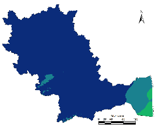
|
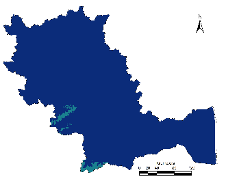
|
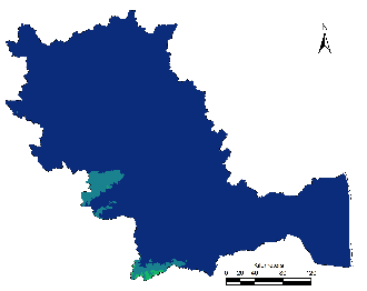
|

|
| January | February | March | April |

|

|

|
|
| May | June | ||
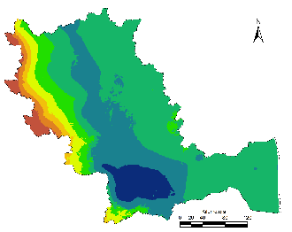
|
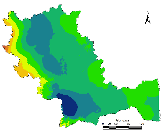
|
||
| July | Annual | August | |
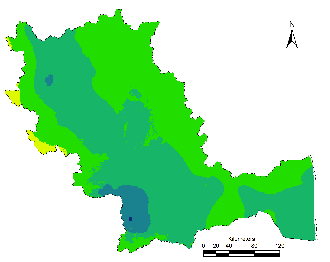
|
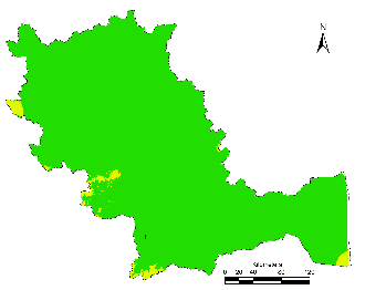
|
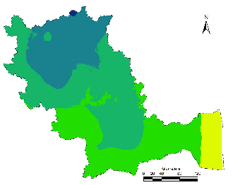
|
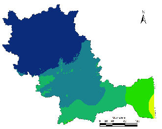
|
| September | October | November | December |
Rainfall (mm)
|
|||
Figure 4.4.17: Rainfall dynamics in Cauvery Basin
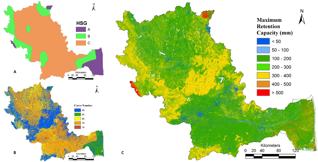
Figure 4.4.18: NRCS parameters (A: Hydrologic Soil Group, B: Curve Number, C: Retention Capacity)
Table 4.4.6 provides yield in basin, and also across the administrative divisions. Karnataka state has an annual water yield of 348TMC of which south west monsoon caters about 68.5% of the total i.e., about 238 TMC and north east monsoon caters to 21% yield, remaining flow is due to the showers during April and May. Tamil Nadu is also equivalent to that of Karnataka yielding water about 325 TMC, Tamil Nadu state receives maximum rainfall during north east monsoon i.e., about 67.7% yielding 220 TMC of water and south west monsoon contributes to 25% of the total yield i.e., about 81 TMC. Kerala contributes to yield of 111 TMC of which south west monsoon contribute to 88.7% of the total yield i.e., about 98.5 TMC. Across the basin, south west monsoon yields 428 TMC and North East Monsoon yields 302 TMC, Gross yield in the basin is about 786 TMC considering non monsoon showers across other months. Estimated annual yield of 786 TMC was found to be comparable with the measurements made by the Cauvery Fact Finding Committee which is about 740 TMC at Lower Anicut [14]. Accuracy of NRCS method to quantify yield was about 93 % based on which the analysis was continued further.

|

|
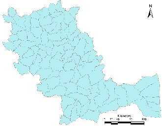
|
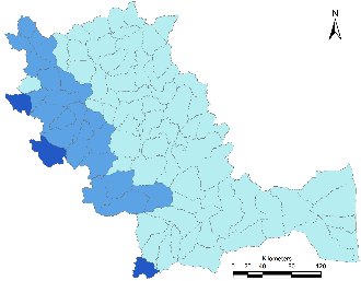
|
| January | February | March | April |
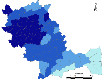
|

|
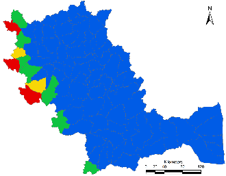
|
|
| May | June | ||
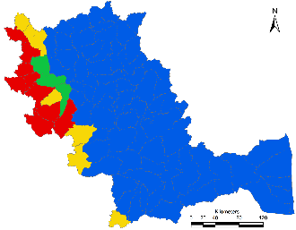
|

|
||
| July | Annual | August | |
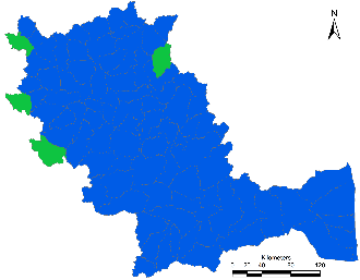
|
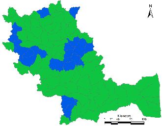
|
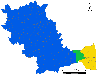
|
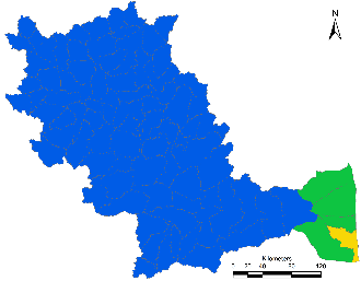
|
| September | October | November | December |
Runoff (mm) 
|
|||
Figure 4.4.19: Sub catchment wise Runoff (mm)
Table 4.4.6: Yield in Cauvery basin across administrative boundaries
|
Yield |
Units |
Kerala |
Karnataka |
Tamil Nadu |
Puducherry |
Basin |
|
South West |
TMC |
98.5 |
238.0 |
81.2 |
0.2 |
418 |
|
North East |
TMC |
7.8 |
72.0 |
220.1 |
1.6 |
302 |
|
Annual |
TMC |
111 |
348 |
325 |
2 |
786 |
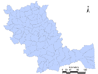
|

|

|

|
| January | February | March | April |
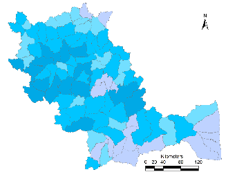
|
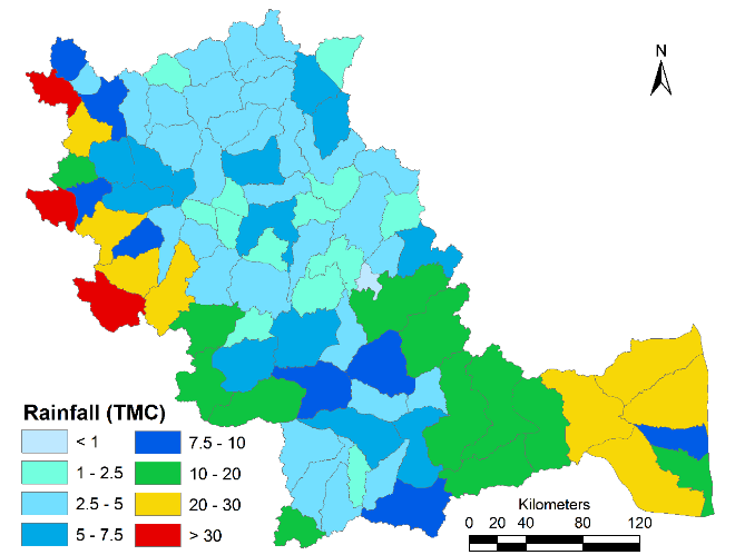
|

|
|
| May | June | ||
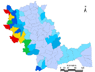
|
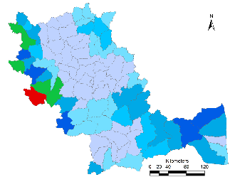
|
||
| July | Annual | August | |
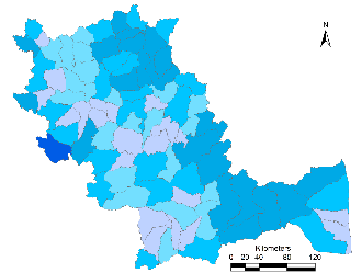
|
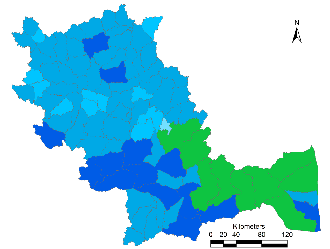
|

|
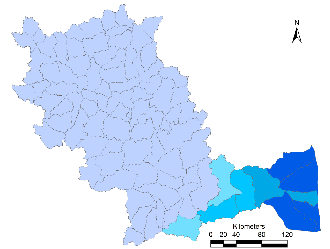
|
| September | October | November | December |
Yield (TMC) 
|
|||
Figure 4.4.20: Sub catchment wise Yield (TMC)
INFILTRATION: Infiltration map across sub catchments of Cauvery is depicted in Figure 4.4.21. The coastal and interior part of Tamil Nadu shows higher infiltration capabilities, which is due to the alluvial soils, followed by the Ghats of Kerala, Karnataka and Tamil Nadu which can be attributed to the presence of Natural vegetation cover.
GROUND WATER RECHARGE: Ground water recharge was quantified based on the lithological conditions in the substrata. Figure 4.4.22, depicts ground water recharge capability across the catchment, indicating that the Ghats and Coast have very high potential of Ground Water Recharging Capability. Across the administrative divisions, Tamil Nadu has highest yield potential about 118 TMC, followed by Karnataka with 109 TMC and Kerala with 41 TMC.
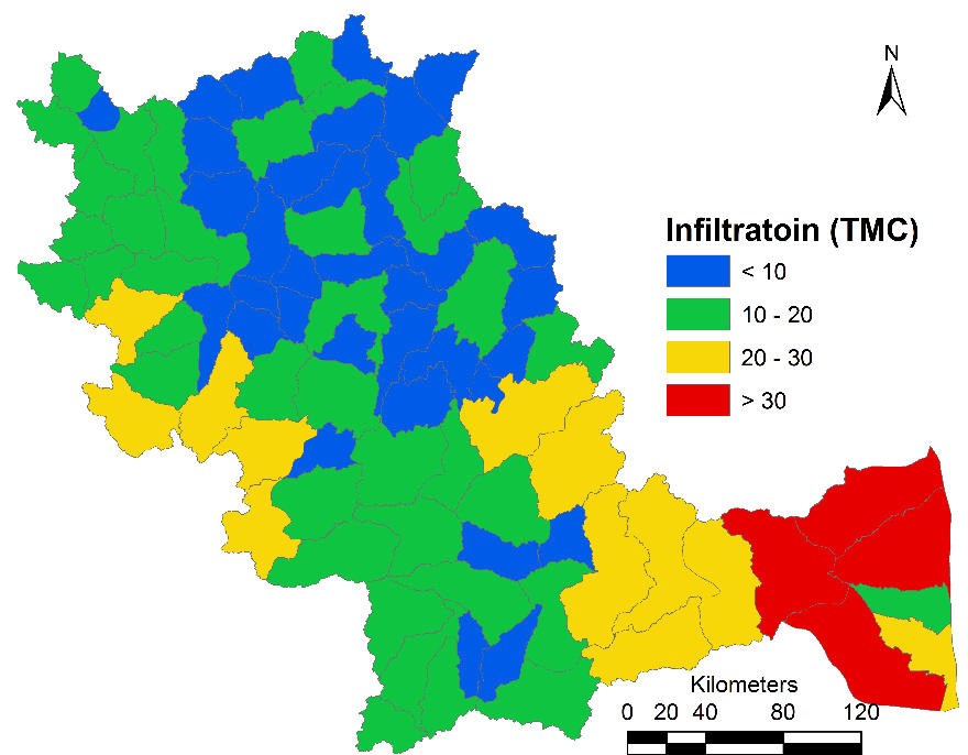
Figure 4.4.21: Infiltration in the basin
|
|
|
|
|
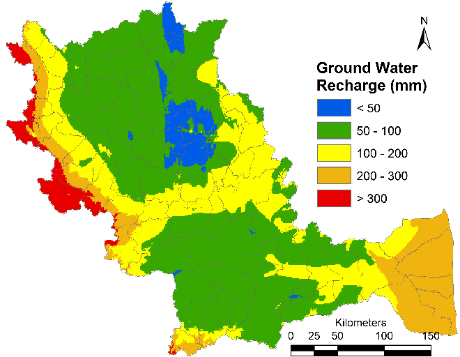

Figure 4.4.22: Ground Water Recharge
EVAPOTRANSPIRATION: Potential Evapotranspiration was quantified using Hargreaves method which considers Temperature variations and solar radiation. Figure 4.4.23 depicts average temperature variations across the basin and Figure 4.4.24 depicts Potential Evapotranspiration as mm/day. Spatial variations in temperature indicates that the Western Ghats have lower temperature as against Eastern Coast and inlands of Tamil Nadu across all months Peak temperatures are observed during the month of April, and lowest during January.
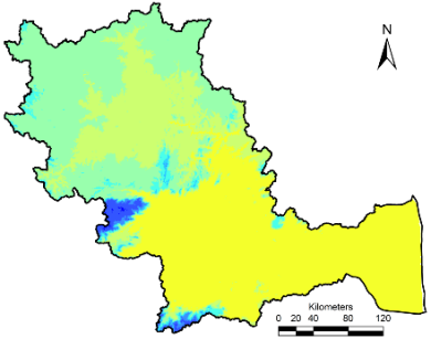
|
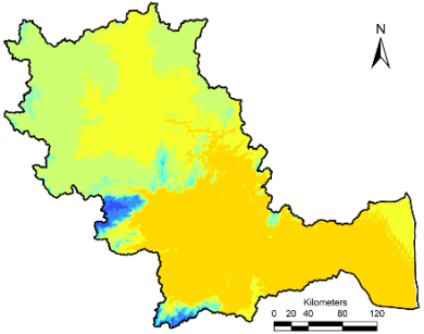
|

|
| January | February | March |
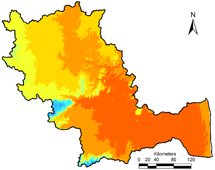
|

|
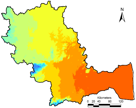
|
| April | May | June |

|

|

|
| July | August | September |

|
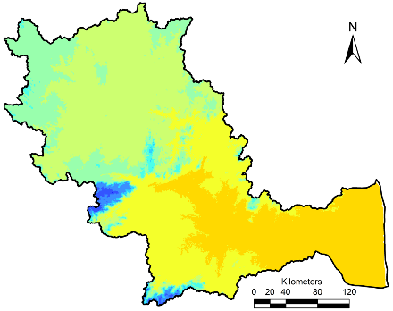
|

|
| October | November | December |
Temperature oC
|
||
Figure 4.4.23: Average Temperature recorded across the basin
Based on the Extra-terrestrial solar radiation, and Temperature across the basin, PET was quantified and is depicted in Figure 4.4.24. PET was found to be high during the months of March, April and May, and Lowest During the Months of November and December

|
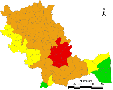
|
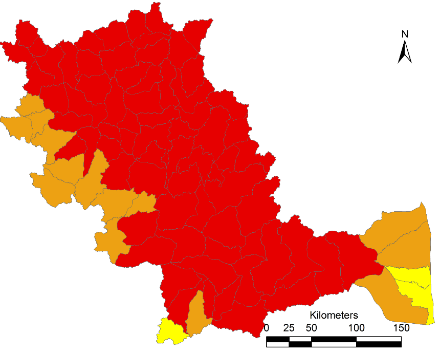
|
| January | February | March |

|
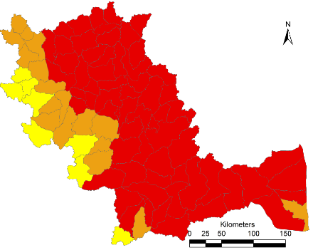
|
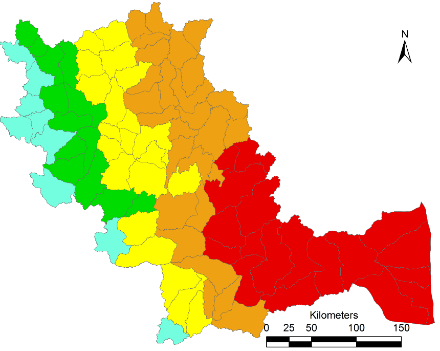
|
| April | May | June |

|
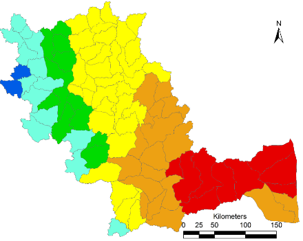
|

|
| July | August | September |
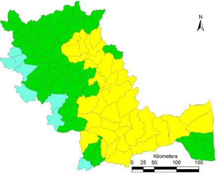
|
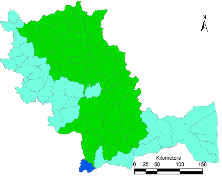
|
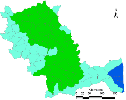
|
| October | November | December |
PET mm/day
|
||
Figure 4.4.24: Potential Evapotranspiration across the basin
Since PET doesn’t consider landscape, AET was quantified, interception losses were deducted to obtain Net AET. Figure 4.4.25 depicts Net AET across the sub catchments of Cauvery.

|
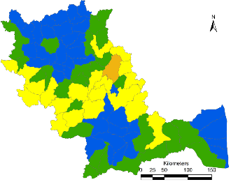
|
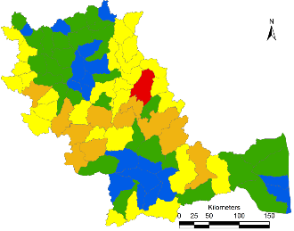
|
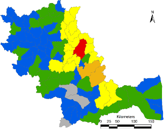
|
| January | February | March | April |

|
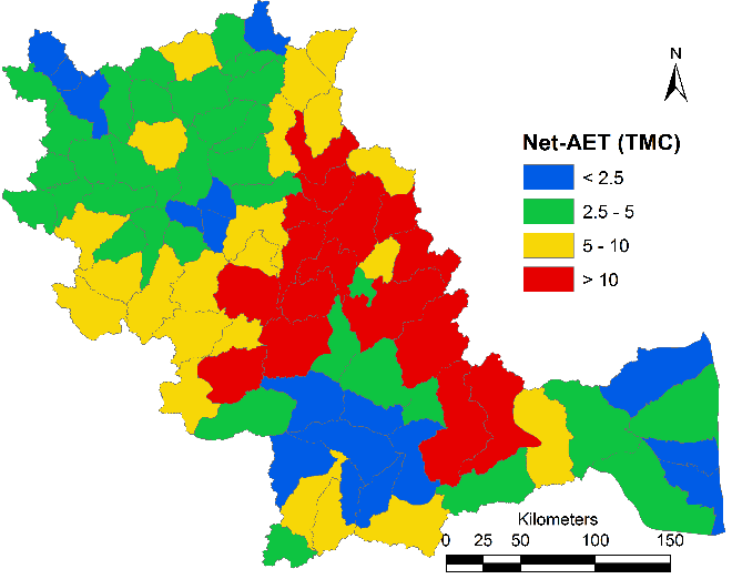
|
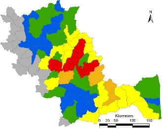
|
|
| May | June | ||
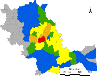
|

|
||
| July | Annual | August | |

|

|
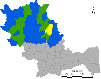
|
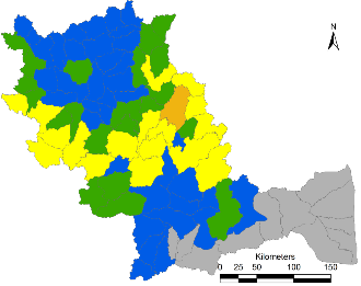
|
| September | October | November | December |
Net AET (TMC) 
|
|||
Figure 4.4.25: Net Actual Evapotranspiration across the basin
4.5 DOMESTIC, LIVESTOCK AND IRRIGATOIN WATER REQUIRMENTS
DOMESTIC WATER DEMAND: Population dynamics across the sub-catchments of Cauvery river is depicted in Figure 4.5.1. Temporal analysis of population indicates that catchments with presence of major cities such as Bangalore, Coimbatore, Salem, Tiruchanapalli and their surrounding have higher population and hence directly proportional to domestic demand (Figure 4.5.2), followed by influence of cities like Mysore, Ramanagar, Chamarajanagar, Thiruppur, Erode, etc.
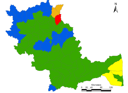
|
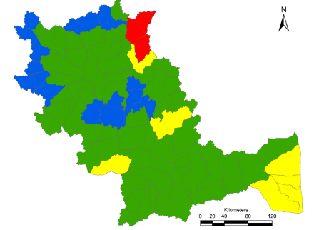
|
| 1991 | 2001 |
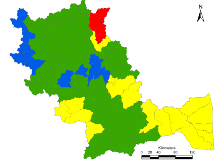
|

|
| 2011 | 2021 |
Population Density (persons/sq.km): 
|
|
Figure 4.5.1: Population dynamics across sub catchment of Cauvery
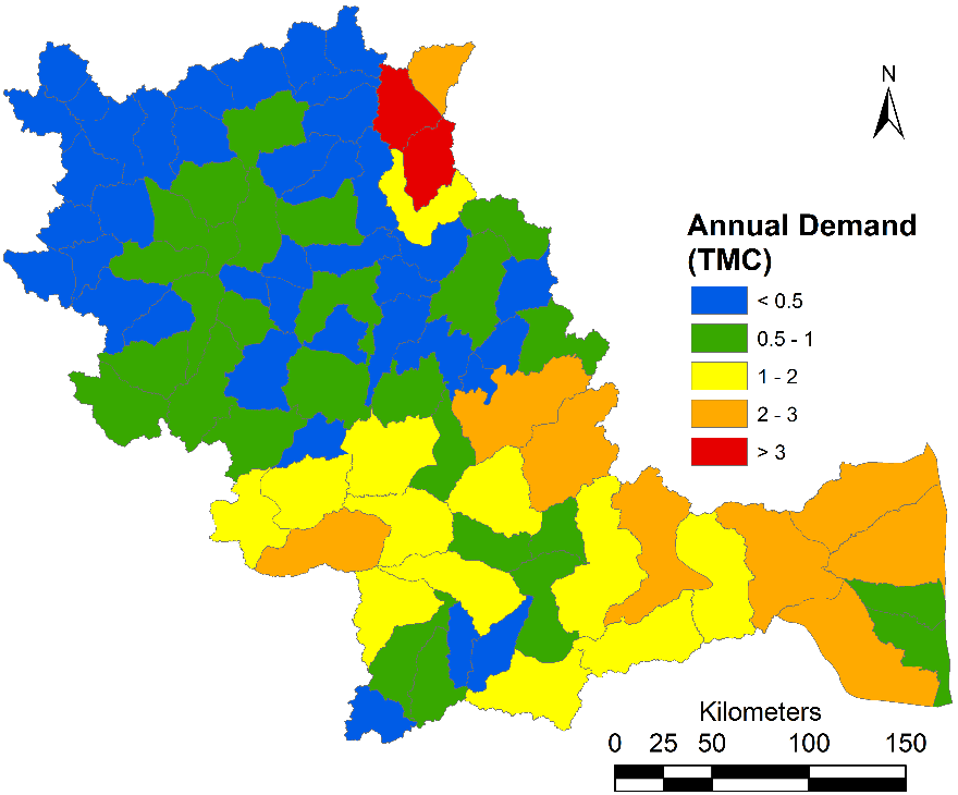
Figure 4.5.2: Domestic Demand (TMC)
Total Domestic Demand in Cauvery basin is about 78 TMC of which Tamil Nadu state has a demand of 45 TMC, Karnataka 30 TMC, Kerala 2 TMC and Puducherry about 1 TMC. Additionally, part of domestic water demand about 180 MLD (2.3 TMC) is catered to Chennai [15] and about 1350 MLD (17.4 TMC) is catered to entire city of Bengaluru [16].
LIVESTOCK WATER DEMAND: Livestock census of different animals and poultry in each district falling under Cauvery basin is depicted in Figure 4.5.3. Cattle and Sheep have highest population followed by Goat and Buffalo. Poultry is higher in administrative division of Tamil Nadu as against Karnataka and Kerala. Spatial distribution of Water Demand (Figure 4.5.4) for Livestock shows that Interior Tamil Nadu demand for water is higher. Across the basin, livestock water demand is about 9 TMC of which Tamil Nadu has a demand of 4.8 TMC, followed by Karnataka with 3.5 TMC and Kerala with 0.1 TMC.
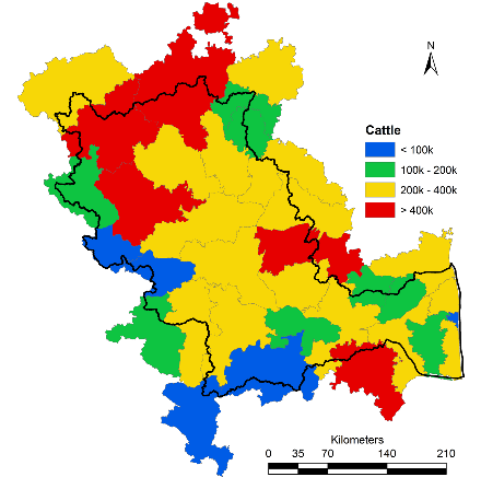
|
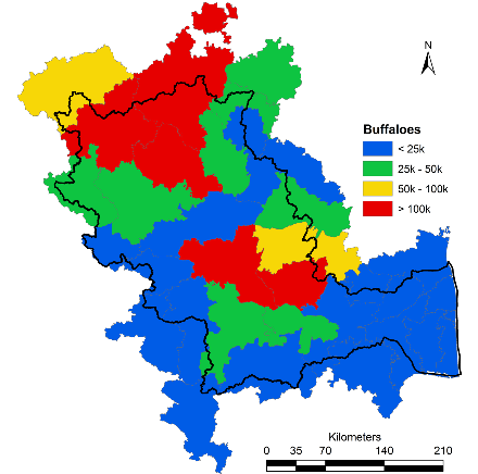
|
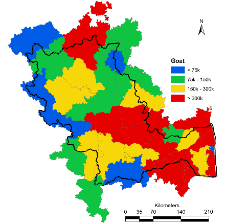
|
| Cattle | Buffalo | Goat |

|

|
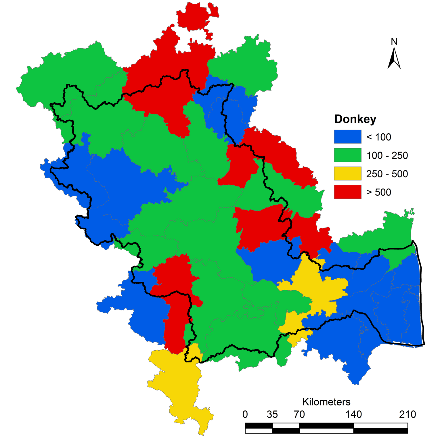
|
| Sheep | Horse | Donkey |

|
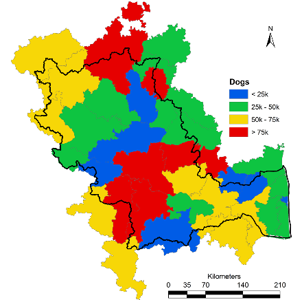
|
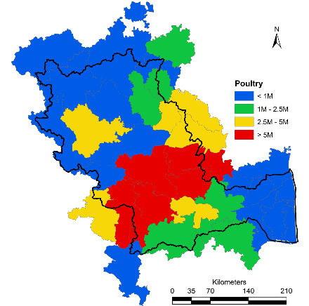
|
| Pig | Dog | Poultry |
Figure 4.5.3: Livestock census across the catchment.
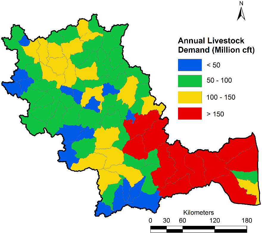
Figure 4.5.4: Livestock Water Demand
AGRICULTURE WATER DEMAND: Area under Major crops across the districts is depicted in Figure 4.5.5 and Table 4.5.1 and Table 4.5.2, crop distribution across the basin at sub catchment level is depicted in Figure 4.5.6.
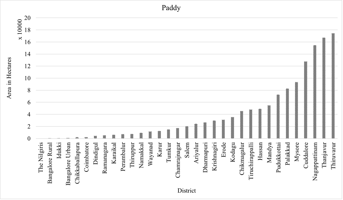
|
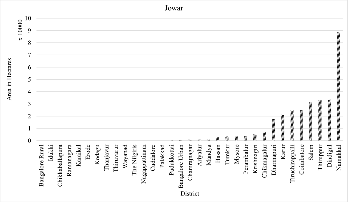
|
| Paddy | Jowar |
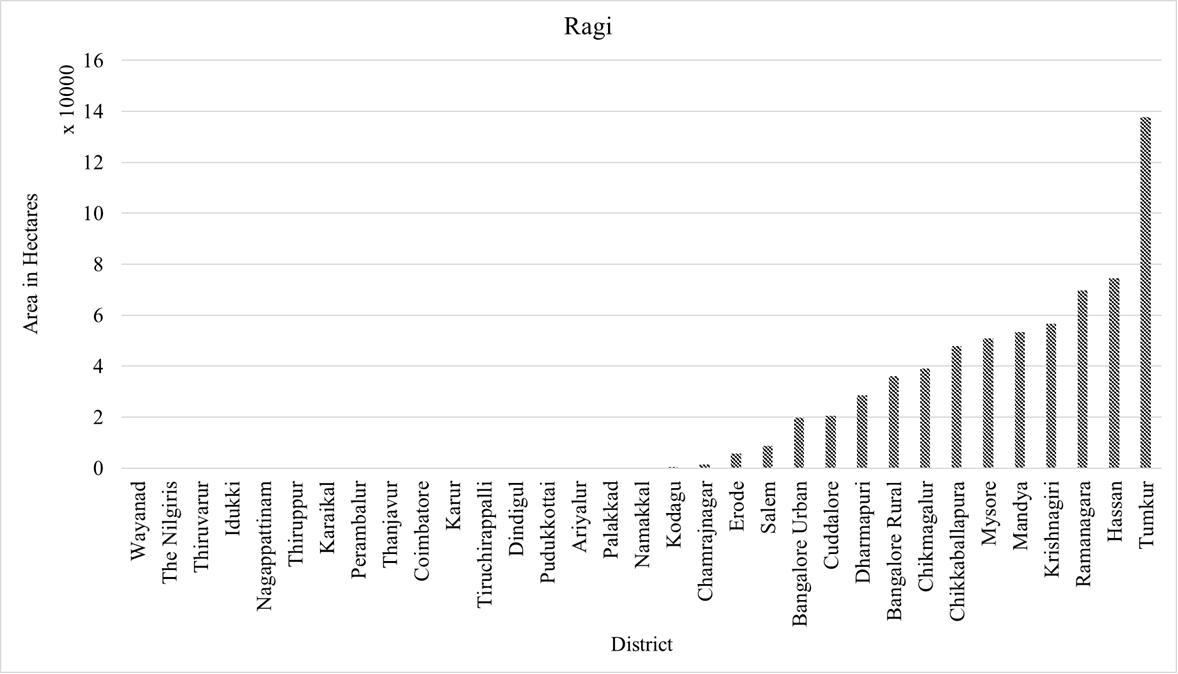
|

|
| Ragi | Maize |

|

|
| Bajra | Other Cereals |
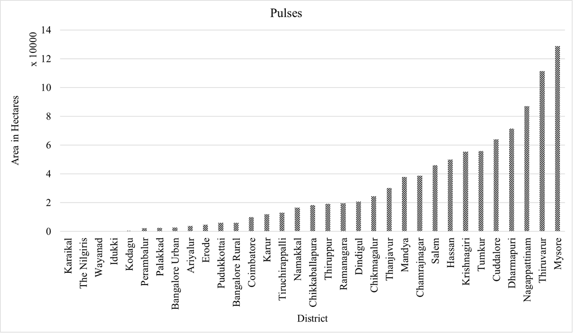
|
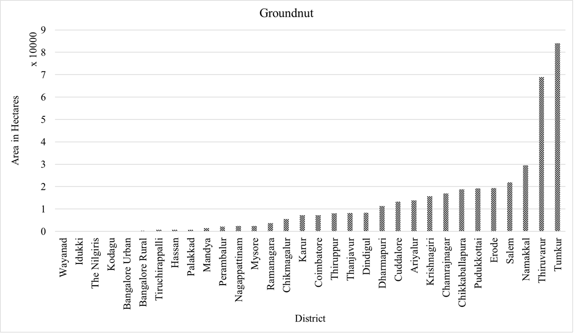
|
| Pulses | Groundnut |
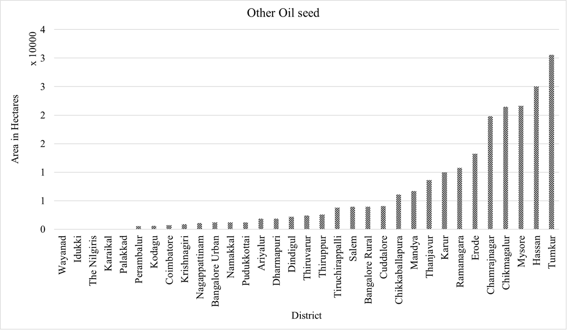
|
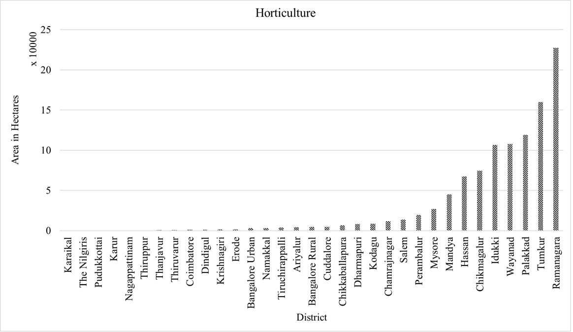
|
| Oilseeds | Horticulture |
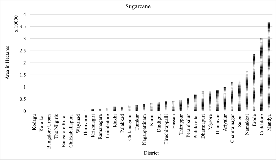
|
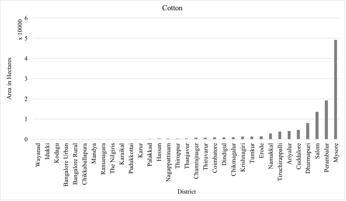
|
| Sugarcane | Cotton |
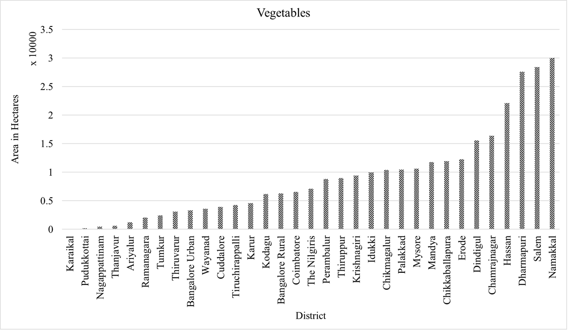
|
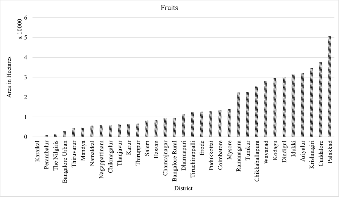
|
| Vegetables | Fruits |
Figure 4.5.5: Area under different crops – district level
Paddy cultivation was dominated in Coastal belt, Ghats and irrigation command area, districts namely Thiruvarur, Tanjavur, Nagipattanam and Cuddalore had paddy fields over 1lakh hectare, followed by Districts of Mysore, Palakkad, Pudukottai and Mandya with area over 50000 hectares. Bajra was dominated in Coastal belt and downstream of Mettur dam. The dry belts were dominated with cereals like Maize and Ragi. Sugarcane cropping was found to be the highest in Mandya, Cuddalore, Erode, Namakar, Salem and Chamrajnagar. Pulses had highest cropping area in Mysore and Thiruvarur, followed by Nagipattanam, Dhamapuri, Cuddalore, Tumkur, Krishnagiri and Hassan Districts. Horticulture crops were found to be highest in Ramanagar and Tumkur with covering over 1.5 lakh hectares followed by Palakkad, Waynad and Iduki with over 1 lakh hectare, Chikkamagalur, Hassan and Mandya with over 40000 hectares.
Table 4.5.1: District wise area under major crops (Cereals and Pulses) – all units in hectares
|
District |
State |
Paddy |
Jowar |
Bajra |
Maize |
Ragi |
Other Cereals |
Pulses |
|
Mysore |
Karnataka |
93521 |
3466 |
0 |
36787 |
50862 |
0 |
128791 |
|
Mandya |
Karnataka |
54847 |
1020 |
0 |
4993 |
53425 |
0 |
37847 |
|
Hassan |
Karnataka |
49317 |
2711 |
43 |
70134 |
74473 |
560 |
49883 |
|
Chikmagalur |
Karnataka |
45286 |
6789 |
0 |
24964 |
39215 |
1182 |
24432 |
|
Kodagu |
Karnataka |
35436 |
0 |
0 |
3273 |
338 |
39407 |
465 |
|
Chamrajnagar |
Karnataka |
17114 |
805 |
135 |
11154 |
1425 |
0 |
38568 |
|
Tumkur |
Karnataka |
14868 |
3334 |
90 |
25191 |
137730 |
2293 |
55833 |
|
Ramanagara |
Karnataka |
5224 |
0 |
3 |
2370 |
69613 |
7 |
19584 |
|
Bangalore Urban |
Karnataka |
807 |
465 |
0 |
1133 |
19713 |
204 |
2623 |
|
Bangalore Rural |
Karnataka |
648 |
0 |
0 |
14558 |
35961 |
17 |
5991 |
|
Palakkad |
Kerala |
82896 |
145 |
0 |
49 |
82 |
40 |
2392 |
|
Wayanad |
Kerala |
11481 |
4 |
0 |
0 |
0 |
0 |
98 |
|
Idukki |
Kerala |
661 |
0 |
0 |
2 |
0 |
3 |
260 |
|
Karaikal |
Puducherry |
6123 |
0 |
0 |
0 |
1 |
0 |
0 |
|
Thiruvarur |
Tamil Nadu |
174366 |
1 |
0 |
1 |
0 |
1 |
111335 |
|
Thanjavur |
Tamil Nadu |
167289 |
0 |
10 |
1475 |
8 |
0 |
30191 |
|
Nagappattinam |
Tamil Nadu |
154750 |
17 |
5 |
22 |
0 |
2354 |
86883 |
|
Cuddalore |
Tamil Nadu |
127485 |
75 |
3559 |
|
20520 |
2032 |
63942 |
|
Pudukkottai |
Tamil Nadu |
72652 |
402 |
21 |
8662 |
35 |
0 |
5981 |
|
Tiruchirappalli |
Tamil Nadu |
48050 |
24608 |
1073 |
9857 |
16 |
2 |
13042 |
|
Erode |
Tamil Nadu |
30889 |
0 |
95 |
18259 |
5626 |
36 |
4702 |
|
Krishnagiri |
Tamil Nadu |
29704 |
4980 |
508 |
3438 |
56649 |
2 |
55441 |
|
Dharmapuri |
Tamil Nadu |
26689 |
17776 |
472 |
13435 |
28607 |
1405 |
71357 |
|
Ariyalur |
Tamil Nadu |
24437 |
872 |
872 |
17768 |
49 |
8 |
3701 |
|
Salem |
Tamil Nadu |
20148 |
31653 |
777 |
35650 |
8626 |
213 |
45940 |
|
Karur |
Tamil Nadu |
12565 |
21225 |
850 |
1804 |
12 |
140 |
11808 |
|
Namakkal |
Tamil Nadu |
9180 |
88750 |
392 |
10029 |
181 |
12679 |
16437 |
|
Thiruppur |
Tamil Nadu |
7511 |
33203 |
43 |
22824 |
0 |
8 |
19175 |
|
Perambalur |
Tamil Nadu |
7175 |
3637 |
191 |
47737 |
1 |
187 |
2252 |
|
Dindigul |
Tamil Nadu |
4234 |
33498 |
750 |
27461 |
16 |
1161 |
20560 |
|
Coimbatore |
Tamil Nadu |
2158 |
25001 |
74 |
5443 |
10 |
1 |
9924 |
|
The Nilgiris |
Tamil Nadu |
328 |
6 |
0 |
0 |
0 |
0 |
1 |
Table 4.5.2: District wise area under major crops(Others) – all units in hectares
|
District |
State |
Fruits |
Vegetables |
Groundnut |
Other Oil seed |
Cotton |
Sugarcane |
Horticulture |
|
Mysore |
Karnataka |
13899 |
10610 |
2387 |
21603 |
49160 |
8435 |
26994 |
|
Mandya |
Karnataka |
4562 |
11785 |
1361 |
6701 |
0 |
36678 |
45023 |
|
Hassan |
Karnataka |
8467 |
22117 |
656 |
25028 |
297 |
4149 |
67106 |
|
Chikmagalur |
Karnataka |
5929 |
10411 |
5557 |
21454 |
1028 |
2426 |
74270 |
|
Kodagu |
Karnataka |
29512 |
6161 |
23 |
572 |
0 |
0 |
8309 |
|
Chamrajnagar |
Karnataka |
9238 |
16414 |
16887 |
19782 |
754 |
11914 |
11696 |
|
Tumkur |
Karnataka |
22335 |
2456 |
83983 |
30549 |
1385 |
2653 |
159998 |
|
Ramanagara |
Karnataka |
22273 |
2036 |
3689 |
10767 |
1 |
1032 |
227352 |
|
Bangalore Urban |
Karnataka |
3049 |
3331 |
72 |
1166 |
0 |
3 |
2771 |
|
Bangalore Rural |
Karnataka |
9592 |
6263 |
297 |
3959 |
0 |
6 |
4614 |
|
Palakkad |
Kerala |
50735 |
10465 |
710 |
31 |
177 |
1874 |
118900 |
|
Wayanad |
Kerala |
28230 |
3585 |
0 |
0 |
0 |
59 |
107797 |
|
Idukki |
Kerala |
31377 |
9939 |
0 |
0 |
0 |
1850 |
106668 |
|
Karaikal |
Puducherry |
16 |
5 |
|
0 |
5 |
1 |
4 |
|
Thiruvarur |
Tamil Nadu |
4278 |
3122 |
68856 |
2374 |
785 |
503 |
785 |
|
Thanjavur |
Tamil Nadu |
6176 |
634 |
8156 |
8614 |
426 |
8580 |
426 |
|
Nagappattinam |
Tamil Nadu |
5773 |
491 |
2386 |
1071 |
317 |
2962 |
317 |
|
Cuddalore |
Tamil Nadu |
37523 |
3950 |
13249 |
4032 |
4630 |
30304 |
4630 |
|
Pudukkottai |
Tamil Nadu |
12738 |
192 |
19143 |
1202 |
13 |
6826 |
13 |
|
Tiruchirappalli |
Tamil Nadu |
12391 |
4240 |
645 |
3756 |
3766 |
4034 |
3766 |
|
Erode |
Tamil Nadu |
12677 |
12246 |
19392 |
13243 |
1421 |
23539 |
1421 |
|
Krishnagiri |
Tamil Nadu |
34572 |
9443 |
15622 |
838 |
1296 |
840 |
1296 |
|
Dharmapuri |
Tamil Nadu |
11292 |
27613 |
11231 |
1858 |
8015 |
8433 |
8015 |
|
Ariyalur |
Tamil Nadu |
32195 |
1212 |
13878 |
1857 |
4074 |
9875 |
4074 |
|
Salem |
Tamil Nadu |
8185 |
28407 |
21939 |
3920 |
13593 |
12652 |
13593 |
|
Karur |
Tamil Nadu |
6446 |
4599 |
7143 |
9960 |
74 |
3372 |
74 |
|
Namakkal |
Tamil Nadu |
5639 |
29989 |
29550 |
1185 |
2816 |
16544 |
2816 |
|
Thiruppur |
Tamil Nadu |
6679 |
8984 |
8035 |
2590 |
335 |
4713 |
335 |
|
Perambalur |
Tamil Nadu |
712 |
8822 |
2096 |
529 |
19231 |
5241 |
19231 |
|
Dindigul |
Tamil Nadu |
29893 |
15563 |
8360 |
2208 |
969 |
3838 |
969 |
|
Coimbatore |
Tamil Nadu |
13532 |
6565 |
7201 |
703 |
948 |
1170 |
948 |
|
The Nilgiris |
Tamil Nadu |
1305 |
7084 |
5 |
0 |
5 |
3 |
5 |
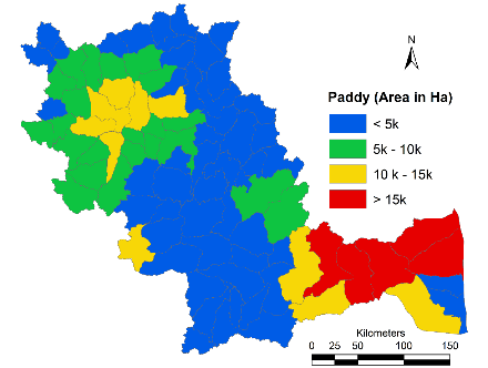
|
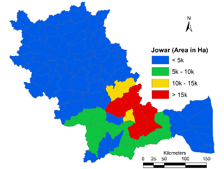
|
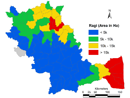
|
|
| Paddy | Jowar | Ragi | |
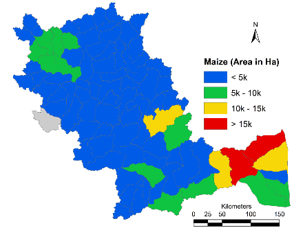
|

|
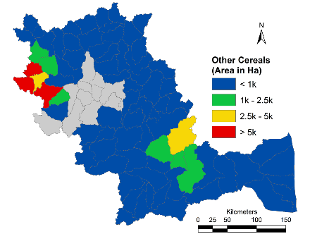
|
|
| Maize | Bajra | Other Cereals | |

|
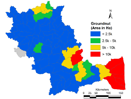
|

|
|
| Pulses | Ground nut | Oil Seeds | |
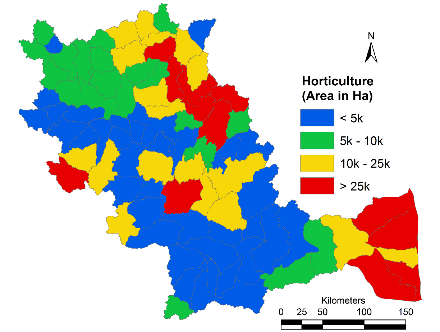
|
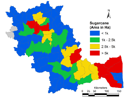
|

|
|
| Horticulture | Sugarcane | Cotton | |
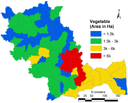
|
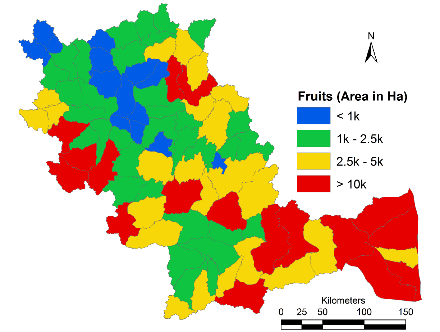
|
||
| Vegetables | Fruits | ||
Figure 4.5.6: Crop Distribution across sub catchments
Agriculture water demand across each sub basin is as presented in Figure 4.5.7. In the existing cropping scenario, Upper Cauvery and Lower Cauvery sub catchments have higher Agriculture water requirement compared to Middle Cauvery sub-catchments. Across the administrative divisions, with existing scenario of cropping, Tamil Nadu has the highest demand of 585 TMC, followed by Karnataka with 529 TMC, Kerala with 62 TMC and Puducherry with 5 TMC. Entire basins water demand with respect to agriculture is about 1180 TMC. Spatial analysis shows that Karnataka and Kerala areas under agriculture depends majorly on South west monsoon between June to September, whereas majority of Tamil Nadu is dependent on the north east monsoon.

|
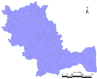
|
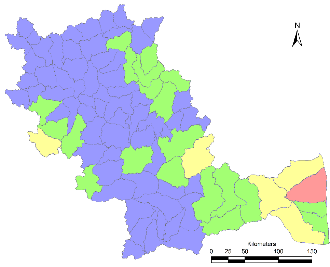
|
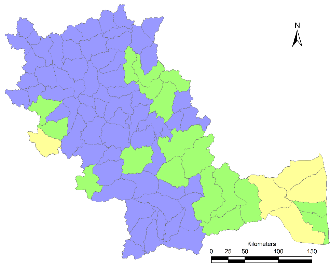
|
| January | February | March | April |
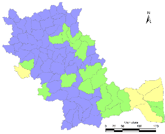
|
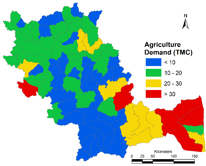
|

|
|
| May | June | ||
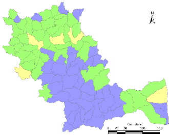
|

|
||
| July | Annual | August | |
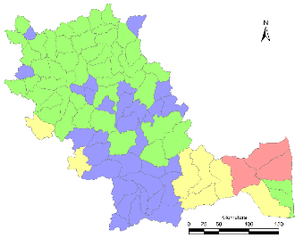
|

|

|
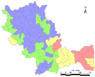
|
| September | October | November | December |
Agriculture Demand (TMC) 
|
|||
Figure 4.5.7: Agriculture Demand in TMC
4.6 HYDROLOGICAL STATUS: Hydrological status was assessed by estimating total demand and Water availability in the catchment. Figure 4.6.1 depicts the total demand across the sub basins. Cauvery basin on a whole has a total demand 1267 TMC of which Tamil Nadu has a demand of 637 TMC followed by Karnataka with 563 TMC, Kerala with 64 TMC and Puducherry with 5 TMC.

|

|
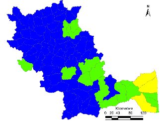
|
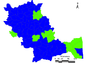
|
| January | February | March | April |
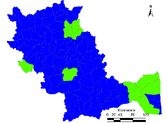
|
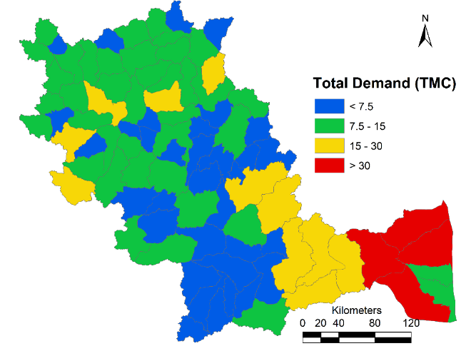
|
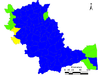
|
|
| May | June | ||
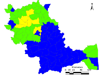
|
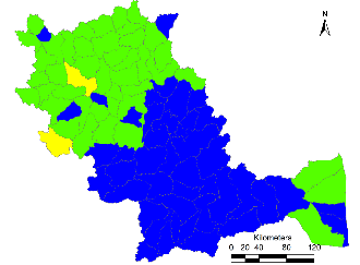
|
||
| July | Annual | August | |

|
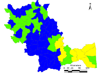
|

|

|
| September | October | November | December |
Total Demand (TMC)
|
|||
Figure 4.6.1: Overall Water Demand in Catchment
Supply is considered as a function of Water yield and Ground water recharge. Hydrological status quantified as function of supply and demand is depicted in Figure 4.6.2. Catchments in the Ghats and closer to the Ghats have better hydrological status with supply greater than 1, whereas the upstream catchment in Karnataka portion of Cauvery indicate severe stresses of water with hydrological status less than 0.5. Interior and Coastal Tamil Nadu portion of Cauvery are also under moderate stresses with existing cropping pattern. On an average the basin has the capability to cater about 67% of the total water requirement with existing cropping pattern and at normal rainfall conditions.
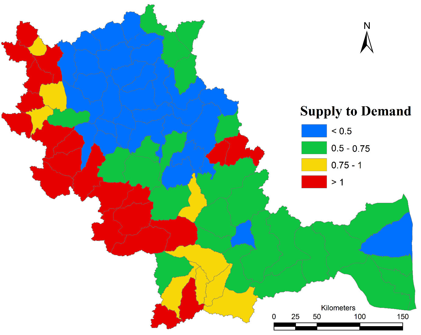
Figure 4.6.2: Hydrological Status
4.7: SCENARIOS
SCENARIO 1: Completely stopping Sugar cane and Grow Paddy instead of sugarcane during monsoons, whereas post monsoon using sugarcane fields for growing low water demanding crops. Based on this condition, the basin demand is about 1004 TMC of which agriculture demand is about 918 TMC. Figure 4.7.1 depicts the hydrological status of Cauvery basin at Scenario 1 condition. Compared to the existing as-usual cropping pattern, in scenario 1, around 83% of the overall demand can be met. Sub catchments towards coast and interior Tamil Nadu shows improvements in hydrological status compared to existing cropping pattern scenario.
SCENARIO 2: The scenario (Scenario 2) is quite similar to the previous scenario (Scenario 1) but with modifications in paddy cultivation i.e., reduction in area under paddy by 50%. Both sugarcane fields and part of paddy fields to be used to grow low water demanding cereals. With this the crop water demand would reduce to 783 TMC and basin water demand to 869 TMC, water demand about 97% can be catered under this scenario. Hydrological status (Figure 4.7.2) shows throughout the basin. Large improvements can be observed in interior and coastal Tamil Nadu, followed by interior Karnataka as against Scenario 1.
|
|
|
|
Figure 4.7.1: Hydrological Status Scenario 1 |
Figure 4.7.2: Hydrological Status Scenario 2 |
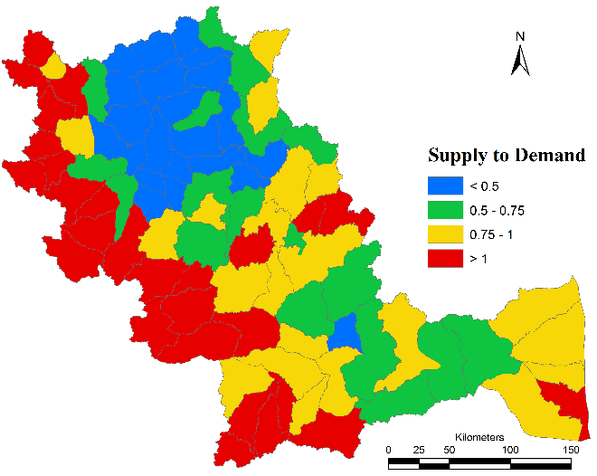
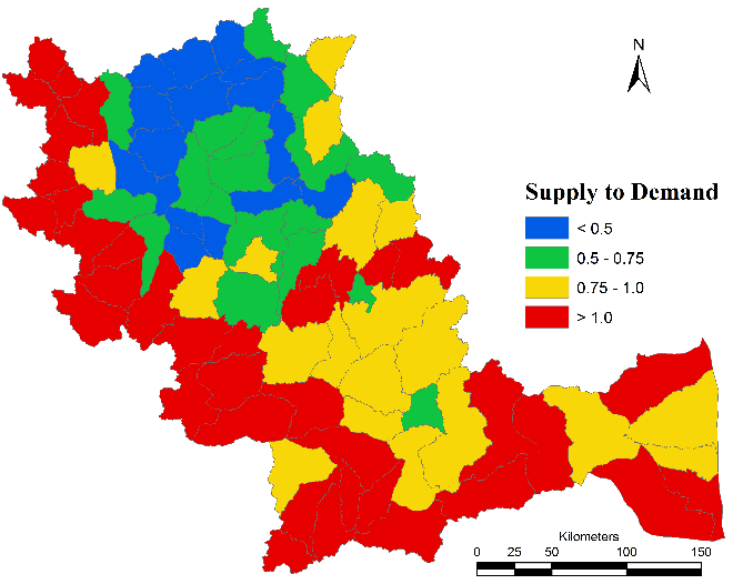
RAINFALL DROUGHT: GPCC data for 113 years was used to estimate COV across Cauvery basin and is depicted in Figure 4.7.3. COV in the basin ranges between 0.12 to 0.28. Low variability (< 15%) of rainfall was observed in the Ghats and High variability (> 25%) at the plains of interior Karnataka. Coast and interior Tamil Nadu had moderate variations about 18 to 22%. Drought rainfall variation across basin and seasons are depicted in Figure 4.7.4. and Figure 4.7.5 depicts the comparison between normal rainfall and drought rainfall. During drought, Rainfall ranges between 364 mm and 4700 mm compared to range of 470 mm to 5500 mm across the basin, on an average, basin receives rainfall of 608 mm. Rainfall distribution across the administrative boundaries is given in Table 4.7.1.
>
Table 4.7.1: Rainfall dynamics across seasons and administrative divisions
|
Rainfall |
units |
Kerala |
Karnataka |
Tamil Nadu |
|
Annual |
mm |
932 |
650 |
554 |
|
South West |
mm |
656 |
368 |
188 |
|
North East |
mm |
149 |
156 |
251 |
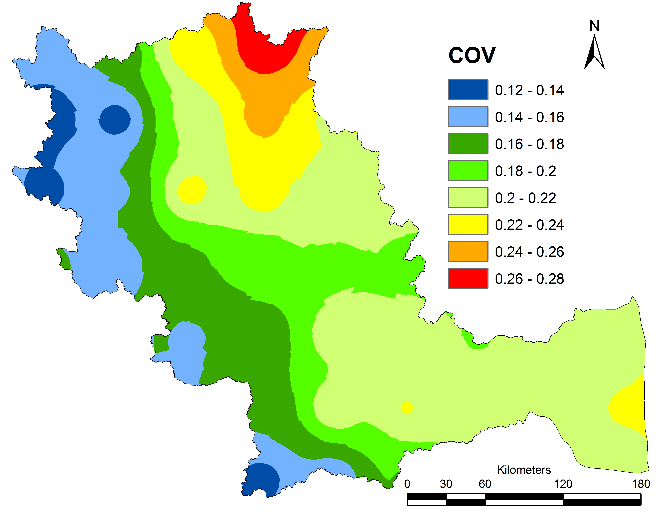
Figure 4.7.3: COV of Rainfall in Cauvery Basin

|
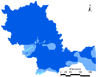
|

|
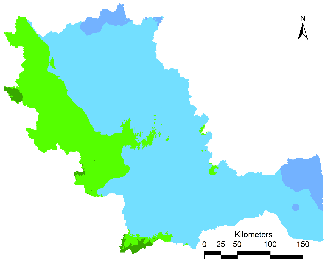
|
| January | February | March | April |
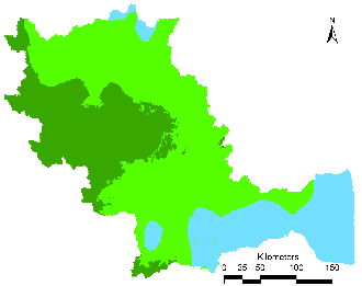
|
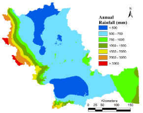
|

|
|
| May | June | ||
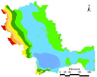
|
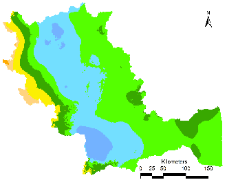
|
||
| July | Annual | August | |
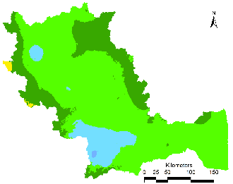
|

|
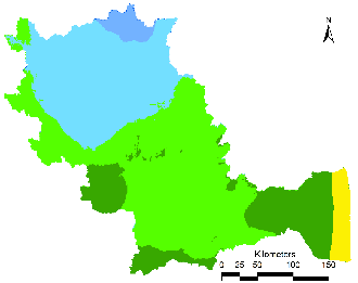
|
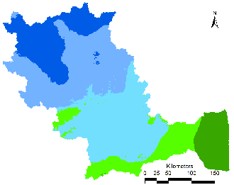
|
| September | October | November | December |
Rainfall (mm) 
|
|||
Figure 4.7.4: Rainfall during Drought Scenario
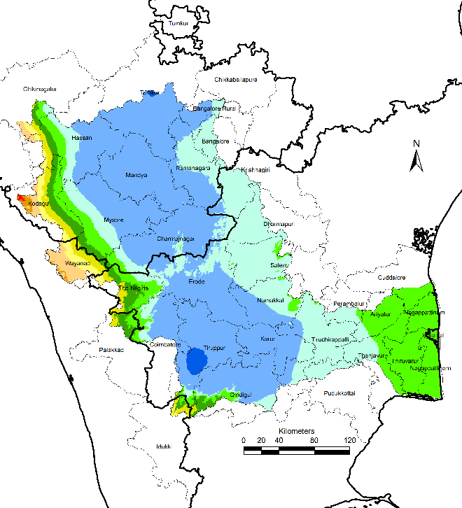
|
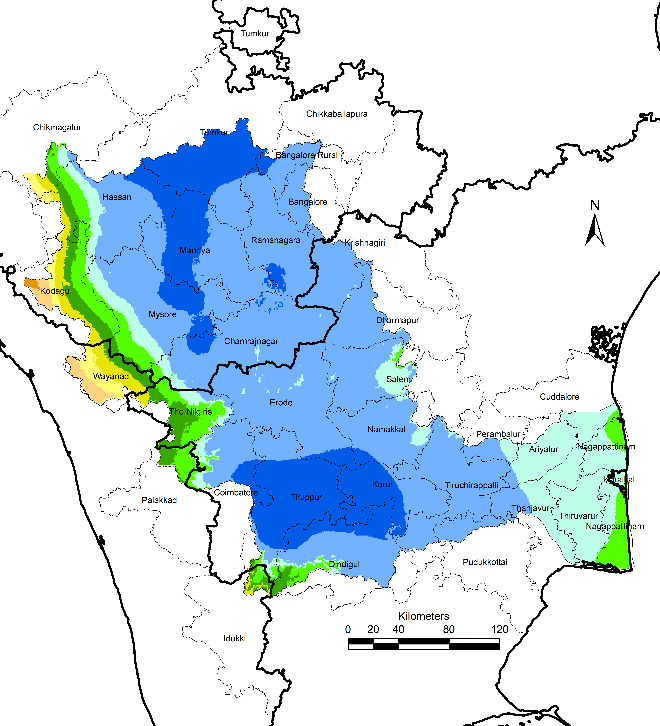
|
| Normal Rainfall | Drought Rainfall |
Rainfall in mm 
|
|
Figure 4.7.5: Comparison of Normal Rainfall and Drought Rainfall
RUNOFF AND YIELD: Estimated runoff in the catchment is depicted in Figure 4.7.6. The coast and the Ghats have higher Runoff volume even during drought years. Annual runoff in the catchment during drought year ranges between 85 mm to 830 mm across the basin. Water yield (Figure 4.7.7) during drought in the catchment is about 535 TMC across the year of which South west monsoons contribute to 302 TMC and North East Monsoons cater to 193 TMC of yield. Across the administrative divisions (Table 4.7.2), Karnataka has yield of about 245 TMC of which South west monsoon has a share of 177 TMC, Tamil Nadu has a water yield of 203 TMC of which North east monsoon contributes 141 TMC, Kerala has a yield of 84 TMC of which South West monsoons cater to 76 TMC.

|
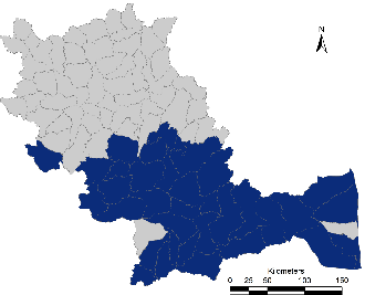
|
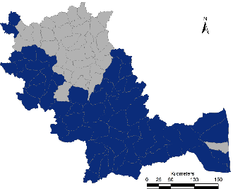
|
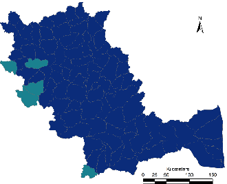
|
| January | February | March | April |

|

|
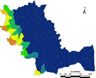
|
|
| May | June | ||
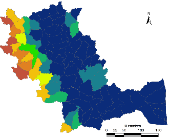
|
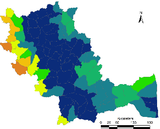
|
||
| July | Annual | August | |

|

|
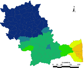
|
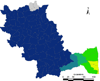
|
| September | October | November | December |
Runoff (mm) 
|
|||
Figure 4.7.6: Runoff during Drought
Table 4.7.2: Catchment Yield during Drought
|
Yield |
Units |
Kerala |
Karnataka |
Tamil Nadu |
Puducherry |
Basin |
|
South West |
TMC |
76.2 |
177.0 |
49.2 |
0.1 |
302 |
|
North East |
TMC |
5.3 |
45.7 |
141.2 |
1.0 |
193 |
|
Annual |
TMC |
84.6 |
245.6 |
203.2 |
1.1 |
535 |
GROUND WATER RECHARGE: Groundwater recharge during drought reduces from 269 TMC to 173 TMC in the basin. Across the catchment, Groundwater recharge in Tamil Nadu portion is about 72 TMC, Karnataka with 69 TMC followed by Kerala with 32 TMC.
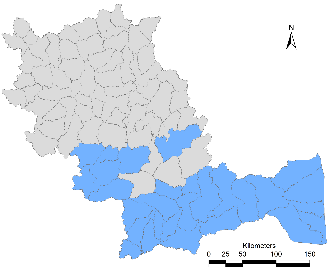
|

|
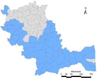
|

|
| January | February | March | April |

|
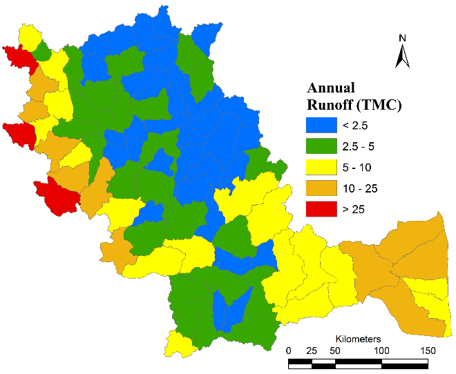
|

|
|
| May | June | ||
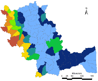
|

|
||
| July | Annual | August | |
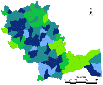
|
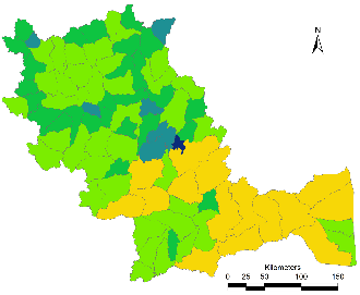
|
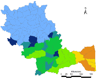
|
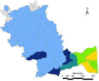
|
| September | October | November | December |
Yield (TMC)
|
|||
Figure 4.7.7: Yield during Drought
Based on basin yield, ground water yield, Scenario 3 and Scenario 4 were formulated.
SCENARIO 3: Since yield during is less than normal, Agriculture pattern was altered based on Scenario 2 condition i.e., by reducing area grown under paddy to 70%, using paddy for millets and other less water demanding cereals. During post monsoons, using these lands for growing pulses and legumes. Other cropping pattern remains same as scenario 2. Total water demand (Figure 4.7.8) in this scenario is about 775 TMC of which agriculture demand is about 689 TMC. Considering annual surface water and ground water yield, about 76% of the total demand can be met.
SCENARIO 4: To ensure best utilization of water available, paddy was completely replaced with less water demanding millets and pulses during monsoon and reducing other crops by 30%. By doing this the total water demand in the basin reduced to 549 TMC against total yield about 558 TMC. Hydrological Status is depicted in Figure 4.7.9, almost all sub basins have lesser stresses compared to scenario 3.
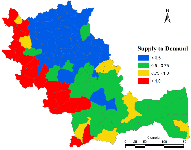
|
| Figure 4.7.8: Hydrological Status- Scenario 3 |
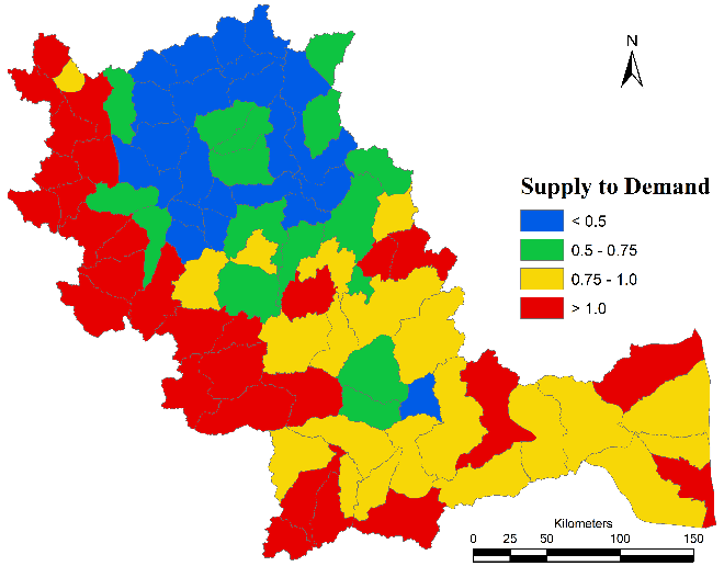
|
| Figure 4.7.9: Hydrological Status- Scenario 4 |
COMPARISON OF SCENARIOS: All the scenarios were compared (Figure 4.7.10) in order to understand the need of various cropping patterns across the sub basins. Table 4.7.3 summarizes the water demand in entire Cauvery Basin. During normal rainfall, highest efficiency can be achieved in Scenario 2, where a during drought conditions, efficiency can be achieved at Scenario 4.
Table 4.7.3: Comparison of Scenarios
| Scenario | Yield TMC | Ground Water Recharge TMC | Domestic Demand TMC | Livestock Demand TMC | Agricultural Demand TMC | Supply to Demand |
| As usual | 786 | 269 | 78 | 9 | 1180 | 67% |
| Scenario 1 | 918 | 83% | ||||
| Scenario 2 | 768 | 97% | ||||
| Scenario 3 | 535 | 173 | 689 | 76% | ||
| Scenario 4 | 462 | 1.02% |
Spatially, across all scenarios, Ghats indicate presence of rich water resource with higher supply than demand, and hence normal cropping pattern can be followed. The other locations sub catchment, for better water utilization can follow Scenario 2, but during drought periods, the non-Ghats basins can adopt, Scenario 4 criteria to ensure sustainable use of water resource.

|
|
| Scenario: As usual Cropping pattern, during Normal Rainfall | |

|

|
| Scenario 1 | Scenario 2 |

|

|
| Scenario 3 | Scenario 4 |
Figure 4.7.10: Hydrological Status comparison across all scenario
4.8: CROPPING PATTERN IN CAUVERY DELTA ACROSS VARIOUS WEATHER CONDITION [17]
Cropping pattern across different seasons and weather conditions across the delta districts of Tamil Nadu (Cauvery Basin) are as described in Tables 4.8.1 to 4.1.6.
Table 4.8.1: Cropping Pattern in Thanjavur District
|
District |
Irrigation System |
Cropping Pattern |
SW Monsoon |
NE Monsoon |
Winter and Summer |
|
THANJAVUR
Rainfall Annual: 1045 mm SW: 342 mm NE : 545 mm |
Command Area |
Existing |
Paddy (SW, NE), Sugar cane (Annual), Gingelly, Pulses, Cotton (Winter & Summer) |
||
|
Normal Rainfall Year |
Paddy (SW, NE), Sugar cane (Annual), Maize (SW), Vegetables (SW), Gingelly, Pulses (SW, Winter & Summer) Cotton, Sunflower (Winter & Summer) |
||||
|
Moderate Drought Year |
Maize (SW), Vegetables (SW), Sweet sorghum (SW), Paddy (NE) Gingelly, Pulses (SW, Winter & Summer) Cotton, Sunflower (Winter & Summer) |
||||
|
Severe Drought Year |
Millets (SW), Gingelly (SW), Maize (NE), Fodder Crops (NE) Pulses (Winter & Summer) |
||||
|
Well Irrigation |
Existing |
Vegetable (SW), Paddy (NE), Ground Nut (Winter & Summer) |
|||
|
Normal Rainfall Year |
Banana (Annual), Onion (SW), Vegetable (SW), Sweet sorghum (SW), Paddy (NE), Maize (SW, Winter & Summer), Pulses, Gingelly (Winter & Summer) |
||||
|
Moderate Drought Year |
Ground nut (SW), Pulses (SW), Fodder Crop (SW), Maize (NE, Winter &Summer), Sunflower, Soybean (Winter & Summer), Gingelly (SW, Winter & Summer) |
||||
|
Severe Drought Year |
Vegetables (SW, NE), Periwinkle, Senna (SW), Pulses (SW), Water melon, Cucumber (Winter & Summer) |
||||
Table 4.8.2: Cropping Pattern in Thiruvarur District
|
District |
Irrigation System |
Cropping Pattern |
SW Monsoon |
NE Monsoon |
Winter and Summer |
|
THIRUVARUR
Rainfall Annual: 1125 mm SW: 302 mm NE : 665 mm |
Command Area |
Existing |
Paddy (SW, NE), Sugar cane (Annual), Gingelly, Pulses (Winter & Summer), Ground nut, Cotton (Winter & Summer) |
||
|
Normal Rainfall Year |
Paddy (SW, NE), Sugar cane (Annual), Maize (SW), Vegetables (SW), Pulses (SW, Winter & Summer) Cotton, Gingelly (Winter & Summer), Sunflower (Winter & Summer) |
||||
|
Moderate Drought Year |
Maize (SW), Vegetables (SW), Sweet sorghum (SW), Paddy (NE) Gingelly, Pulses (SW, Winter & Summer) Cotton, Sunflower (Winter & Summer) |
||||
|
Severe Drought Year |
Millets (SW), Gingelly (SW), Maize (NE), Fodder Crops (NE) Pulses, Sunflower (Winter & Summer) |
||||
|
Well Irrigation |
Existing |
Vegetable (SW), Paddy (SW, NE), Ground Nut (Winter & Summer) |
|||
|
Normal Rainfall Year |
Vegetable (SW), Sweet sorghum (SW), Paddy (NE) Ground nut, Maize (SW, Winter & Summer), Pulses, Gingelly (Winter & Summer) |
||||
|
Moderate Drought Year |
Ground nut (SW), Fodder Crop (SW), Pulses (SW), Maize (SW, NE, Winter &Summer), Sunflower, Soybean (Winter & Summer), Gingelly (SW, Winter & Summer) |
||||
|
Severe Drought |
Pulses (SW, NE, Winter and Summer) Gingelly (SW) |
||||
Table 4.8.3: Cropping Pattern in Trichirapalli District
|
District |
Irrigation System |
Cropping Pattern |
SW Monsoon |
NE Monsoon |
Winter and Summer |
|
TRICHIRAPALLI
Rainfall Annual: 759 mm SW: 270 mm NE : 356 mm |
Command Area |
Existing |
Paddy (SW, NE), Sugar cane (Annual), Gingelly, Pulses (Winter & Summer), Ground nut, Cotton (Winter & Summer) |
||
|
Normal Rainfall Year |
Paddy (SW, NE), Sugar cane (Annual), Maize (SW), Vegetables (SW), Pulses (SW, Winter & Summer) Cotton, Gingelly (Winter & Summer), Sunflower (Winter & Summer) |
||||
|
Moderate Drought Year |
Maize (SW), Vegetables (SW), Sweet sorghum (SW), Pearl Millet (SW), Fodder Sorghum (SW), Paddy (NE) Gingelly, Pulses (SW, Winter & Summer) Senna, Coleus (Winter & Summer), Flower Crops (Winter & Summer) |
||||
|
Severe Drought Year |
Millets (SW), Gingelly (SW), Maize (NE), Pulses (Winter & Summer) |
||||
|
Well Irrigation |
Existing |
Vegetable (SW), Paddy (SW, NE), Ground Nut (Winter & Summer) Banana (Annual) |
|||
|
Normal Rainfall Year |
Banana (Annual), Gloriosa (Annual), Flower Crops (Annual), Onion (SW), Coleus (SW), Vegetable (SW), Sweet sorghum (SW), Paddy (NE) Maize (SW, Winter & Summer), Ground nut, Pulses (Winter & Summer), Gingelly (Winter & Summer) |
||||
|
Moderate Drought Year |
Fodder Crop (SW), Pulses (SW), Maize (SW, NE), Sunflower, Soybean (Winter & Summer), Sorghum, Gingelly (Winter & Summer) Ground nut (Winter & Summer) |
||||
|
Severe Drought Year |
Vegetables (All seasons) Periwinkle, Senna (SW) Watermelon (Winter & Summer) |
||||
Table 4.8.4: Cropping Pattern in Perambalur District
|
District |
Irrigation System |
Cropping Pattern |
SW Monsoon |
NE Monsoon |
Winter and Summer |
|
PERAMBALUR
Rainfall Annual: 949 mm SW: 349 mm NE : 449 mm |
Command Area |
Existing |
Paddy (SW, NE), Sugar cane (Annual), Gingelly, Pulses, Onion (Winter & Summer), Ground nut, Cotton (Winter & Summer) |
||
|
Normal Rainfall Year |
Paddy (SW, NE), Sugar cane (Annual), Maize (SW), Vegetables (SW), Onion, Pulses (Winter & Summer) Cotton, Gingelly (Winter & Summer), Sunflower (Winter & Summer) |
||||
|
Moderate Drought Year |
Maize (SW), Vegetables (SW), Sweet sorghum (SW), Pearl Millet (SW), Fodder Sorghum (SW), Paddy (NE) Gingelly, Pulses (SW, Winter & Summer) Senna (All Seasons) Periwinkle, Coleus (Winter & Summer), |
||||
|
Severe Drought Year |
Millets (SW), Gingelly (SW), Maize (NE), Fodder Crop (NE) Pulses (SW, Winter & Summer) |
||||
|
Well Irrigation |
Existing |
Vegetable (SW), Paddy (SW, NE), Ground Nut (Winter & Summer) Gingelly (Winter & Summer) Sugarcane, Banana (Annual) |
|||
|
Normal Rainfall Year |
Sugarcane, Banana, Gloriosa (Annual), Flower Crops (Annual), Onion (SW), Coleus (SW), Vegetable (SW), Sweet sorghum (SW), Maize (SW), Paddy (NE), Ground nut, Pulses (Winter & Summer), Gingelly (Winter & Summer) |
||||
|
Moderate Drought Year |
Fodder Crop (SW), Pulses (SW), Maize (SW), Cotton (NE) Sunflower, Soybean (Winter & Summer), Sorghum, Gingelly (Winter & Summer) Ground nut (Winter & Summer) |
||||
|
Severe Drought Year |
Vegetables (All seasons) Periwinkle, Senna (SW) Watermelon (Winter & Summer) |
||||
|
Rain fed |
Existing |
Gingelly, Sorghum (SW, NE), Maize, Millet (SW, NE) Pulses, Coriander (Winter & Summer) Cotton, Ground nut (Winter & Summer) |
|||
|
Normal Rainfall Year |
Gingelly, Sorghum (SW, NE), Maize, Millet (SW, NE) Pulses, Coriander (Winter & Summer) Cotton, Ground nut (Winter & Summer) |
||||
|
Moderate Drought |
Cotton (SW, NE), Gingelly (SW, NE), Pulses (NE to Winter & Summer) |
||||
|
Severe Drought |
Fodder, Sorghum, Minor Millets, Coriander (NE to Winter & Summer) |
||||
Table 4.8.5: Cropping Pattern in Pudukottai District
|
District |
Irrigation System |
Cropping Pattern |
SW Monsoon |
NE Monsoon |
Winter and Summer |
|
PUDUKOTTAI
Rainfall Annual: 917 mm SW: 349 mm NE : 418 mm |
Command Area |
Existing |
Paddy (SW, NE), Sugar cane (Annual), Gingelly, Pulses, Onion (Winter & Summer), Ground nut, Cotton (Winter & Summer) |
||
|
Normal Rainfall Year |
Paddy (SW, NE), Sugar cane (Annual), Gingelly, Pulses, Onion (Winter & Summer), Ground nut, Cotton (Winter & Summer) |
||||
|
Moderate Drought Year |
Maize (SW), Vegetables (SW), Sweet sorghum (SW), Pearl Millet (SW), Fodder Sorghum (SW), Paddy (NE) Pulses (SW, Winter & Summer) Ground nut, Gingelly (Winter & Summer) Coleus (Winter & Summer), |
||||
|
Severe Drought Year |
Millets (SW), Gingelly (SW), Maize (NE), Fodder Crop (NE) Pulses (SW, Winter & Summer) Periwinkle, Senna (NE) |
||||
|
Tank Irrigation |
Existing |
Paddy (SW, NE), Ragi (NE) Ground Nut, Pulses (Winter & Summer) |
|||
|
Normal Rainfall Year |
Paddy (SW, NE), Ragi (SW) Vegetables (SW) Ground nut, Pulses (Winter & Summer),
|
||||
|
Severe Drought Year |
Fodder Crop, Water Melon, Cucumber (NE) |
||||
|
Well Irrigation |
Existing |
Banana, Sugarcane (Annual), Ground nut (SW), Ragi (SW) Paddy (NE) Pulses (Winter & Summer) |
|||
|
Normal Rainfall Year |
Banana, Sugarcane (Annual) Ground nut (SW), Ragi (SW) Sweet Sorghum (SW), Maize (SW, NE), Paddy (NE) Pulses, Gingelly (Winter & Summer) |
||||
|
Moderate Drought Year |
Ground nut, Ragi (SW) Fodder crop (SW), Maize (NE) Water Melon, Pulses (Winter & Summer) |
||||
|
Severe Drought Year |
Fodder, Sorghum, Minor Millets, (NE to Winter & Summer) |
||||
|
Rain fed |
Existing |
Ground nut, Red gram, Ragi (SW, NE) Castor (SW), Millet (NE) |
|||
|
Normal Rainfall Year |
Ground nut, Red gram, Ragi (SW, NE) Castor (SW), Millet (NE) |
||||
|
Moderate Drought Year |
Pulses (SW), Ragi (SW, NE) Oil Seeds (SW, NE) |
||||
|
Severe Drought Year |
Fodder, Pulses, Millets, Oil Seeds, Cucurbits (SW,NE) |
||||
Table 4.8.6: Cropping Pattern in Cuddalore (Chidambaram and Kattumannarkovil) District
|
District |
Irrigation System |
Cropping Pattern |
SW Monsoon |
NE Monsoon |
Winter and Summer |
|
CUDDALORE
Rainfall Annual: 1248 mm SW: 373 mm NE : 716 mm |
Command Area |
Existing |
Paddy (All Seasons), Sugar cane (Annual), Gingelly, Pulses (Winter & Summer), Ground nut, Cotton (Winter & Summer) |
||
|
Normal Rainfall Year |
Paddy (All Seasons), Sugar cane (Annual), Maize, Vegetables (SW) Gingelly, Pulses (SW, Winter & Summer), Ground nut, Cotton (Winter & Summer) |
||||
|
Moderate Drought Year |
Maize (SW), Vegetables (SW), Sweet sorghum (SW), Fodder Sorghum (SW), Paddy (NE) Pulses (Winter & Summer) Gingelly (Winter & Summer) |
||||
|
Severe Drought Year |
Millets (SW, NE), Maize (NE), Gingelly (Winter & Summer), Perennial Trees (Fruits and Timber) |
||||
Controversy due to Mismanagement of Catchment
|
Controversy - Causes |
|
|

Figure 5.1: Area under irrigation in the Cauvery Basin [1]
|
|
|
|
|
|
Area under irrigation is depicted in Figure 5.1 and increase in the area is given in Table 5. 1. Figure 5.2 depicts the trend in the increase in area under irrigation. During 1901 and 1928 irrigation area in Tamil Nadu was 6556 sq.km and Karnataka had about 1193 sq.km and there was no increase in irrigation area across Karnataka and Tamil Nadu. However, there was a drastic increase during the subsequent period.
- Post 1991 to 2014: 9000 sq.km increase in Tamil Nadu and 5500 sq.km in Karnataka;
- 1956 and 1971: 1000 sq.km increase in Tamil Nadu and 600 sq.km in Karnataka;
- 1928 – 1956: increase of about 2800 sq.km in Tamil Nadu and about 1000 sq.km in Karnataka.
During the last century, area under irrigation area has increased from 6556 sq.km (13.8%) to 20233 sq.km (42.7%) in Tamil Nadu and 1193 sq.km (3.42%) to 8497 sq.km (24.32%) in Karnataka part of Cauvery.

Figure 5.2: Irrigation Area dynamic’s in Cauvery basin [1]–[4]
Table 5.1: Temporal dynamics in irrigation area– Cauvery basin [1]–[4]
|
Year |
Tamil Nadu |
Karnataka |
||
|
Hectares |
Percentage |
Hectares |
Percentage |
|
|
1901 |
655614 |
13.8 |
119340 |
3.42 |
|
1928 |
655614 |
13.8 |
119340 |
3.42 |
|
1956 |
934857 |
19.7 |
210444 |
6.02 |
|
1971 |
1139890 |
24.1 |
271341 |
7.77 |
|
Current* |
2023300 |
42.7 |
849700 |
24.32 |
Dispute [1]–[4], [7] - Genesis
- Lack of integrated river basin management and understanding of hydrologic regime;
- Genesis of Cauvery problem is since 1892 and 1924 - Agreements between Madras Presidency and Princely State of Mysore.
- 1892 Agreement between Madras Presidency and Princely State of Mysore, allowing Mysore to take up irrigation.
- 1924, agreement between two governments (lapse after run of 50 years)
- After independence in 1954, Kodagu came under Mysore state, Madras Presidency was further divided to Tamil Nadu and Kerala States. The changes brought conflict in water distribution since Kabini tributary lies in Kerala.
- Agriculture area increase 6500 sq.km (Tamil Nadu) and 1193 sq.km (Karnataka) in 1924 to 20000 sq.km (Tamil Nadu) and 8497 sq.km (Karnataka) in current decade.
- Water allocation during normal rainfall regime is reasonable, whereas during droughts allocation of same quantity of water to the riparian states is gross mismanagement.
Figure 5.3 depicts the unrealistic allocation by The Cauvery Water Dispute Tribunal, due to the lack of understanding of the hydrologic process and on flawed assumptions. Currently Tamil Nadu is allotted about 419 TMC, followed by Karnataka with 270 TMC and Kerala with 30 TMC, about 10 TMC as natural flow.

Figure 5.3: Water Allocation as per Cauvery Water Dispute Tribunal [2]
Irrigation demand and domestic demand since 1900 in Kerala, Karnataka and Tamil Nadu is as depicted in Figure 5.4 and Table 5.2. Escalations in the water Demand due to intense cropping has increased from 502 TMC in 1901 to 749 TMC in 1971, reducing the environmental flow needs. Water allocations between the administrative divisions are based on demand of water for intense irrigation rather than the availability. The Tribunal as per its judgment indicates only 10 - 14 TMC of water as Environmental water demand.
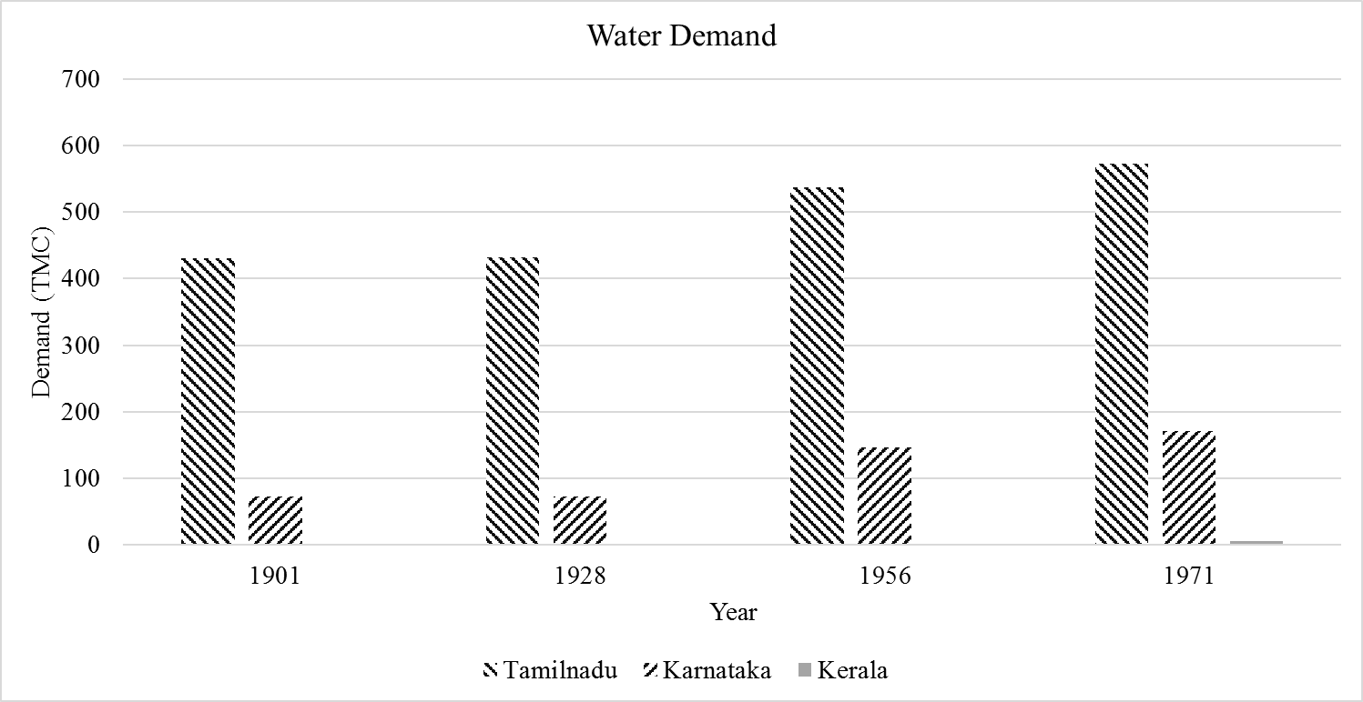
|
|
||||||||||||||||||||
|
Figure 5.4: Water Demand in TMC [2] |
Table 5.2: Water Demand (TMC) |
Cauvery basin - Water Sharing Agreements
- 1872 First inter-state water-sharing agreement between Mysore and the Madras Presidency
- 1892 Agreement between Madras Presidency and Princely State of Mysore, allowing Mysore to take up irrigation.
- 1924, agreement between two governments (lapse after run of 50 years)
- 1954, post-independence, Kodagu came under Mysore state, Madras Presidency was further divided to Tamil Nadu and Kerala States. The changes brought conflict in water distribution since Kabini tributary lies in Kerala.
- 1924 Second water-sharing agreement for the next 50 years
- 1960 Karnataka proposes and builds four reservoirs
- 1970 Cauvery Fact Finding Committee set up in anticipation of the ending of the agreement in 1974. Its final report came in 1976 which was accepted by all the states. But when Karnataka began construction of the Harangi dam, Tamil Nadu went to court
- 1980 Litigations, conflicts and negotiation between the parties continue
- 1990 Supreme Court directs the Centre to constitute Cauvery Water Dispute Tribunal (CWDT)
- 1991 CWDT announces an interim award. Orders Karnataka to release water. In a move to nullify the interim awards, the Karnataka government passes an ordinance "to protect" irrigation in the "irrigable areas" of the Cauvery. Supreme Court strikes down the ordinance; upholds the CWDT award.
- 1993 Tamil Nadu Chief Minister demands the state's share as stipulated by the interim order
- 1998 Centre constitutes Cauvery River Authority to ensure implementation of the interim award of CWDT
- 2002 Cauvery River Authority chaired by Prime Minister directs Karnataka to release 9,000 cusecs of water to Tamil Nadu.
- 2005 Karnataka refuses to implement the distress-sharing formula
- 2007 CWDT gives final award, calling the agreements of 1872 and 1924 executed between Madras and Mysore as valid. Karnataka protests
- 2015 Tamil Nadu Chief Minister writes to Prime Minister of India, requesting him to advise Karnataka to release water. Karnataka refuses to release water since it is a "distress year"
- 2016 The Supreme Court asks Karnataka to consider releasing water to Tamil Nadu to help the state continue to "exist as an entity".
- 2018 the Cauvery Water Management Authority (CWMA) as per the Supreme Court order and constitution of The Cauvery Water Regulation Committee
GROUND WATER TABLE FLUCTUATIONS
Ground water data table variations after monsoons and in summers were analyzed based on data collated from the Central Ground Water Board [5], [6] between 1996 and 2016, based on 146 ground water observation wells whereas in Cauvery Middle sub-basin there are 612 observation wells located and Cauvery upper sub-basin comprises of 115 observation wells. Figure 5.5 depicts over 1200 Ground water observation stations maintained by CGWB within the basin. Ground water table dynamics across the catchment during post monsoon season and summer season is as depicted in Figures 5.6 and 5.7 respectively.
Ground water table during the post monsoon varies between less than 2.5 m to over 20 m whereas the ground water depth exceeds between 10 m to over 40 m during the summer season across the Cauvery river basin. This emphasizes that sufficient groundwater is available in the Deccan plateau and there is a need to adopt water efficient crops during the post monsoon period.
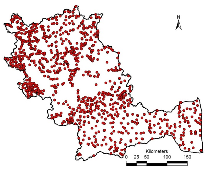
|

|
|
Figure 5.5: Ground water table observation stations |
Figure 5.6: Ground water table – Post monsoon |
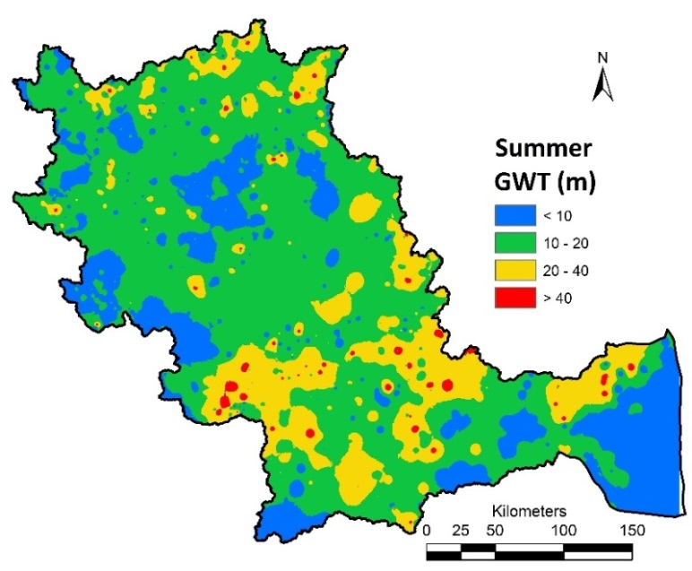
|
|
|
Figure 5.7: Ground water table - Summer |
|
Figures 5.8 and 5.9 depict district wise ground water dynamics during monsoon and summer seasons respectively. Across seasons, deltas indicate higher water table across all seasons varying between < 1 meter to just over 10 m. Districts such as Coimbatore, Bangalore have deeper ground water tables (over 20 m) during Summer followed by districts namely Erode, Karur, Namakal, Ariyalur, Salem, Dharmapuri, Krishnagiri, Bangalore, and Tumkur with ground water table between 15 to 20 meters.
Annual Ground water variations are depicted in Figure 5.10, and spatial distribution of COV at district level is as represented in Figure 5.11. COV ranges from 0.25 to 0.66 across the districts. Over exploited blocks depict higher ground water variability between seasons. Similarly, the Coastal zones and portion of Plains in Tamil Nadu, and Karnataka have lower variations.
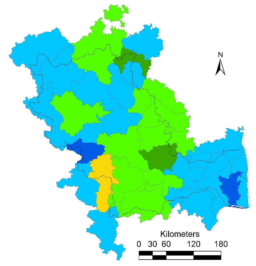

Figure 5.8: District wise Ground water dynamics across Cauvery basin – Monsoon
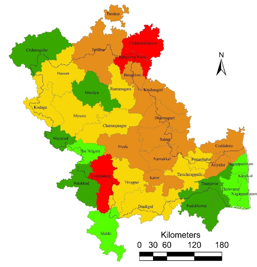
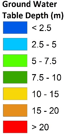
Figure 5.9: District wise Ground water dynamics across Cauvery basin – Summer
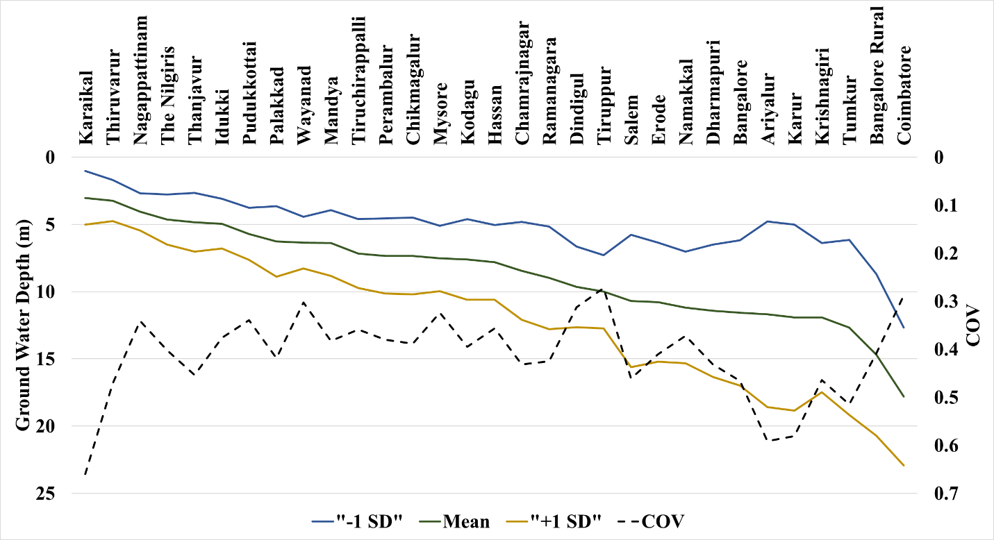
Figure 5.10: Ground Water Table Dynamics (Average ± Standard Deviation, COV)
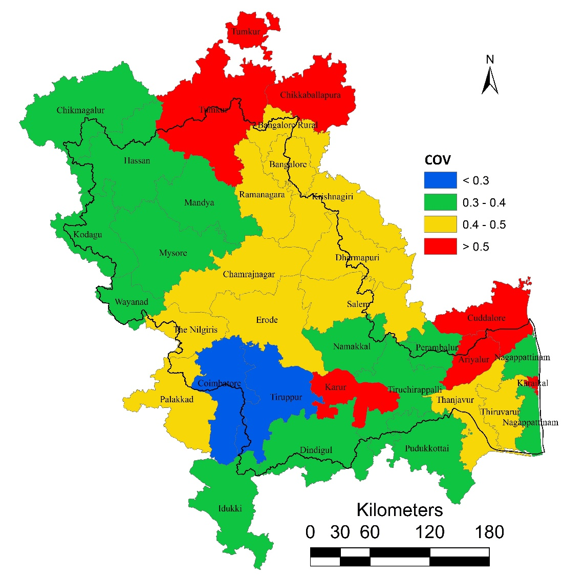
Figure 5.11: COV – Ground Water
Recommendations
Major threats to the sustenance of water in the Cauvery basin are unabated deforestation process, changes in the climate due to global warming, and water vulnerability leading to shortages with impacts on drinking water supply and the future of adequate food production. Hence, sound management system has become imperative, as the very real threats of climatic changes further exacerbate the problem of dwindling water supply. This entails
- Arresting deforestation in Cauvery catchment, through afforestation of native
species (funds available under CAMPA (Compensatory Afforestation Management and
Planning Authority) funds, GoI, could be used for this purpose); native vegetation
has a multitude of effects in catchments: the presence of native vegetation can
influence local
rainfall in complex and unexpected ways and that land clearing can lead to a reduction in
rainfall (Western Ghats). Native vegetation protection and rehabilitation are also important to other aspects of the hydrological cycle, including sub-surface flow, groundwater recharge, base flow and maintaining riparian vegetation. - First responsibility is to protect and improve the catchment area through forestation. This would substantially enhance the quantity and quality of water in the river basin. Earlier studies in the Western Ghats have shown that wherever the forest cover is high, stream network is also good and healthy. High sedimentation would result on account of lack of forest cover. This would aggravate the supply of water against the ever increasing demand for it. Second, it is necessary to prioritise drinking water requirement. National Water Policy of the Government of India recognizes water for drinking and sanitation as the pre-emptive needs. Finally, people should be educated on the use and abuse of water; short of these, all efforts through agitations will go waste in the long run.
- Allocation of CAMPA funds for Rejuvenation of Cauvery catchment through location specific watershed management to ensure a sustainable method of water resource usage. Advantages of proper utilization of watersheds: Help slow down the process of surface water run-off, Improve percolation of water to recharge underground aquifers, Decrease the siltation of waterway and help lengthen the flow period of rivers.
- Desilting of all lakes, tanks and ponds in the Cauvery catchment on priority; Need to reintroduce the AncientNeerkatti concept of constructing, maintaining and managing the water harvesting structures at decentralized levels under MNREGA (The Mahatma Gandhi National Rural Employment Guarantee Act 2005 Ministry of Rural Development, Government of India). Livelihood in Indian villages is centered on water and agriculture. For example, in the downstream of Cauvery basin, water harvesting structures were kept well through ‘Kudimaramathu’ - participation by villagers to keep all the physical structures intact and ways were devised and a dedicated “Neerkatti‟ monitor water levels and was in charge of channeling this water to individual fields and to retain the incoming water based on the requirement of the village and the excess was allowed to flow into the next tank in the series.
- Removal of accumulated sediment in the reservoirs;
- Land use changes, groundwater pumping and diversions all affect river flows, so the focus must be on an equitable sharing of all the water, and not just the surface flow in the river.
- Scientific investigations and data collection of basin hydrology, ecosystems, and human and legal aspects of water management. This science-based approach would minimize conflicts and enhance collaboration.
- Scientific approach to protect catchment areas, increasing forest and grassland covers, adopting appropriate cropping pattern consistent with soil characteristics and finally, opting for systematic silt management in the reservoirs and ponds can provide some good sensible solutions to water scarcity problems, and not simply harping on river diversions as the ultimate solution.
- Appropriate cropping with identification of cropping zones, seasonal versus annual versus perennial (plantations) crops
- Water use efficiency: Adopting drip irrigation technology in Cauvery basin as it will provide significant external and private benefits to farmers by lowering dependency on river as well as ground water resources. Water management policy of the various states fall in the basin should provide attention on the promotion of drip irrigation in where water and labor scarcity are critical. The state governments should take proactive encouragement of technology adoption through incentive programs as potential for conservation.
- Sustainable Allocation of water based on availability and prioritization of use
- Stopping the Illegal Soil Excavation and Sand Mining: The river bed of Cauvery is subjected to soil excavation and sand mining activities in certain areas, though these activities are restricted by the respective department. These activities have resulted in lowering of riverbed level as well as river water level and also resulting in lowering of groundwater table due to excessive extraction and draining out of groundwater from the adjacent areas. The soil excavation will reduce the thickness of the natural filter materials (Top layer soil), infiltration through which the ground water is recharged. These activities induce soil runoff during monsoon season resulting in siltation in the rivers also collapse or landslide of the adjacent structures and variation in river slope and flow velocity. As these activities are posing a threat to the river, concerned departments should take stringent actions against these activities by regularly monitoring. Sand mining was observed with in 300m buffer zone of Cauvery river in villages like Nelliya hadakeri, Keralapur, Kannambadi (Venugopala temple), Maralagala (Dodddapalya), Mahadevapura and Somanthapur, Purigali, Harale and Dhanagere.
- Removal of all encroachments of River bed and natural drains (streams)
- Setting up common effluent treatment plants and ensure zero Industrial Effluent Discharge into the River Course.
- Integrated Management of the catchment irrespective of Cultural, Linguistic and Political dimensions.
- Implementation of National Water Policy: recognizes that development and management
of water resources need to be governed by national perspectives in order to develop
and conserve the scarce water resources in an integrated and environmentally sound
basis. The major provisions under the policy are:
- Envisages to establish a standardized national information system with a network of data banks and data bases
- Resource planning and recycling for providing maximum availability
- To give importance to the impact of projects on human settlements and environment.
- Regulate exploitation of groundwater
- Setting water allocation priorities in the following order: Drinking water, Irrigation, Hydropower, Navigation, Industrial and other uses.
- The water rates for surface water and ground water should be rationalized with due regard to the interests of small and marginal farmers.
- The policy also deals with participation of farmers and voluntary agencies,
in maintaining water quality, water zoning, conservation of water, flood and
drought management, erosion etc.
The other major features are:- - To ensure access to a minimum quantity of potable water for essential health and hygiene to all citizens, available within easy reach of the household.
- To curtail subsidy to agricultural electricity users.
- Setting up of Water Regulatory Authority.
- To keep aside a portion of the river flow to meet the ecological needs and to ensure that the low and high flow releases correspond in time closely to the natural flow regime.
- To give statutory powers to Water Users Associations to maintain the distribution system.
- Project benefited families to bear part of the cost of resettlement & rehabilitation of project affected families.
- To remove the large disparity between stipulations for water supply in urban areas and in rural areas.
- To support a National Water Framework Law.
- There is an urgent need for an expert independent body to address this intricate issue and examine the ground realities.
- Share should be in proportion to the water yield in the catchment (spatial extent) and also the extent of forest cover in the region.
- River basin to be treated as an integrated ecosystem and should not be based on language, political boundary or any such unscientific criteria.
- Four different allocation strategies are: (1) maintaining minimum flow levels at state lines (or other useful gauging stations), (2) approaches based on reservoir storage, (3) formulas allocating fixed or percentage-based rights to consumption or diversion, and (4) a requirement—for upstream states to deliver downstream a minimum volume (rather than a constant flow rate) over a lengthy period.
- The principle of natural justice should be employed to protect both the upper and lower catchments of the river, while prioritizing drinking water supply as a priority. Trans-boundary water disputes can be defined broadly, occurring whenever demand for water is shared by any sets of interests, be they political, economic, environmental, or legal. Conflicts over shared water resources occur at multiple scales, from sets of individual irrigators, to urban versus rural uses, to users located in different political jurisdictions.
- Need to establish the federal joint commission (on the lines of successful
model of International Joint Commission to address water conflicts between USA
and Canada) for preventing and resolving disputes. An unbiased,
scientifically based, inclusive, and open to public input, joint commission can
alert the governments to emerging issues that might have negative impacts on the
quality or quantity of boundary waters and brings to the attention of senior
officials the latest developments in science, engineering, and administration
that could benefit the management, security, or conservation of water related
natural resources. The commission needs to be an impartial, quasi-adjudicatory
body and the regulator of projects that affect levels and flows on both sides
of the boundary and as a nonbinding advisor to the governments on controversial
issues relating to both water quantity and quality. The involvement of local
populations in decision-making regarding natural resources can improve the planning
process on all scales. The responsibilities of the commission shall be
- Better land use planning, floodplain mapping and forecasting, to address the challenges of climate changes with the global warming, which will enhance the pressure on water supplies in arid areas and there will be enhanced competition for already limited water supplies and all water-using sectors;
- Preventing or minimizing water loss in the catchment through return fow and implementation of environmentally sound water conservation measures;
- No significant adverse individual or cumulative impacts to the quantity or quality of the Waters and water-dependent natural resources;
- An improvement to the waters and water-dependent natural resources; and compliance with the applicable local, federal, and national laws and policies;
- Integrated land and water resources management and conservation to reduce risk and uncertainty and sustain national and regional development.
- Establish joint mechanisms and capacity to identify risk and uncertainty issues related to (i) land use change in recharge areas and humid zones, (ii) climate change with reduced net
- recipitation, and (iii) inappropriate development, extraction and surface based water pollution and salinization.
- Establish mechanisms to formulate policies for management of identified risk and uncertainty issues, and establish a legal and institutional cooperative framework.
Annexure
Flora diversity of Cauvery River Basin:
The flora diversity of Cauvery Basin is documented by reviewing various literature. The review has covered trees, shrubs, herbs in various locations of basin accounting 2102 entries. The floral species (486) covered under 116 families across the basin in 118 locations. The Lauraceae, Fabaceae, Myrtaceae, Poaceae, Rubiaceae are dominant families found in the basin. The region has highly endemic species around (147 species) such as Artocarpus hirsutus, Atalantiawightii, Blachia umbellate, Cinnamomum macrocarpum, Cinnamomum malabaricum, Cinnamomum travancoricum, Diospyrouspaniculata, Garcinia gummi-gutta, Holigarnagrahamii, Hopea ponga, Ixora brachiata, Knema attenuate, Pinanga dicksonii, Syzygiumdensiflorum, Syzygiummalabaricum, Terminalia travancorensis, Vateria indica etc.
Faunal diversity of Cauvery River Basin:
The faunal diversity of Cauvery Basin is documented by reviewing various literature covering entire region. The review has covered faunal species such as fish, amphibians, birds, insects, butterfly, mammals etc., in various locations of basin accounting 3033 entries. Total 781 species under 184 families were recorded in which, 52 species of fishes under 12 families, 10 species of crabs under 6 families, 74 species of amphibians under 10 families, 80 species of reptiles under 19 families, 388 bird species under 88 families, 51 butterflies under 9 families, 27 insects under 9 families, and 99 mammalian species under 31 families.
District Wise Details :
Cauvery Landscape Dynamics
CAUVERY LANDSCAPE DYNAMICS since 1984 to 2017 (Google Earth)
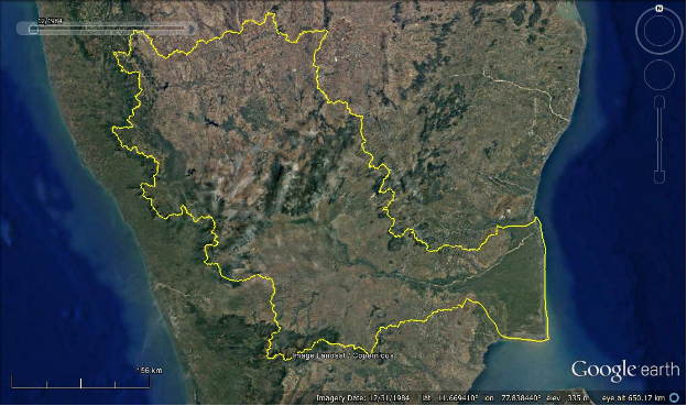
Figure 1: Google Earth 1984

Figure 2: Google Earth 1995

Figure 3: Google Earth 2005
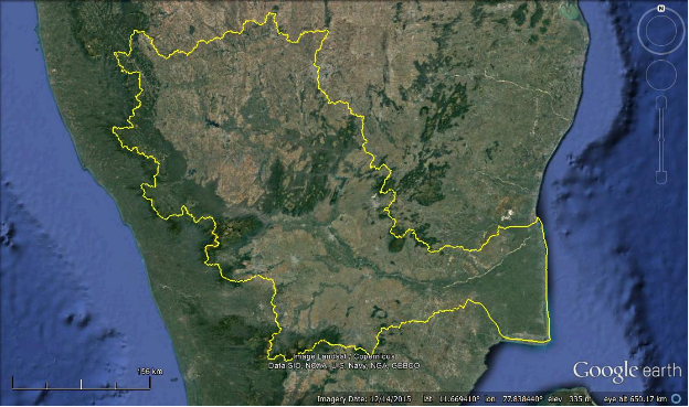
Figure 4: Google Earth 2015
Developmental Activities in the Cauvery Basin
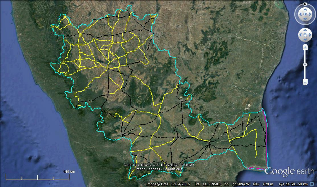
Figure 5: Major Road Network
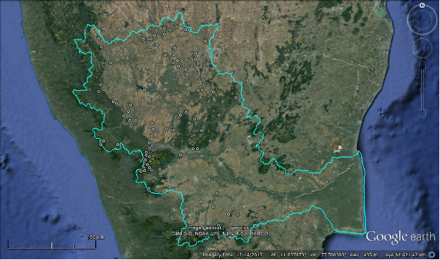
Figure 6: Reservoirs and Dams
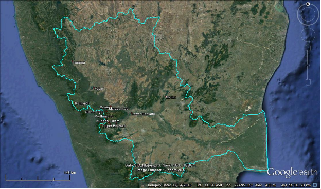
Figure 7: Hydro Electric Power Projects
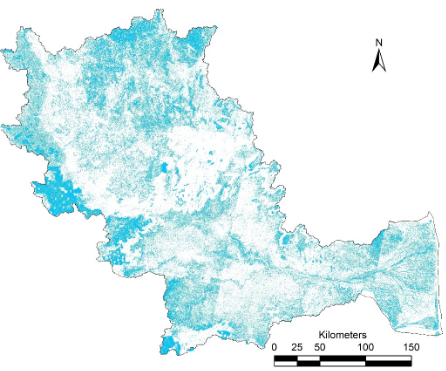
Figure 8: Monoculture
References
RESEARCH HIGHLIGHTS :
[1] Ramachandra T V , Vinay S, Bharath S and Bharath H A, 2020., Cauvery River: Land use dynamics and Hydrological Status, ENVIS Technical Report 161, Sahyadri Conservation Series 90, Environmental Information System, CES, Indian Institute of Science, Bangalore
INTRODUCTION :
[1] WWF GLobal, “Water as a natural resource.” [Online]. Available: http://wwf.panda.org/about_our_earth/teacher_resources/webfieldtrips/water/. [Accessed: 18-Oct-2017].
[2] T. Oki and S. Kanae, “Global Hydrological Cycles annd World Water Resources,” Science (80-. )., vol. 313, no. 5790, pp. 1068–1072, 2006.
[3] Natural Resources of Canada, “Earth Sciences Water,” Government of Canada. [Online]. Available: http://www.nrcan.gc.ca/earth-sciences/science/water/10814. [Accessed: 18-Oct-2017].
[4] European Space Agency, “Global Land cover 2010,” 2012. [Online]. Available: http://www.esa.int/spaceinimages/Images/2014/10/Land_cover_2010. [Accessed: 18-Oct-2017].
[5] Committee on Challenges and Opportunities in the Hydrologic Sciences; National Research Council, Challenges and Opportunities in the Hydrologic Sciences. Washington DC: National Academies Press, 2012.
[6] I. A. Shiklomanov, “World Fresh Water Resources,” in Water in Crisis: A Guide to the World’s Fresh Water Resources, Peter H Ge., Oxford University Press, 1993, p. 473.
[7] International Water Centre, “The Brisbane Declaration,” 2007. [Online]. Available: http://www.watercentre.org/news/declaration. [Accessed: 18-Oct-2017].
[8] P. H. Gleick, “Basic water requirements for human activities: Meeting basic needs,” Water Int., vol. 21, no. 2, pp. 83–92, 1996.
[9] S. K. Jain, “Assessment of environmental flow requirements for hydropower projects in India,” Curr. Sci., vol. 108, no. 10, pp. 1815–1825, 2015.
[10] P. Tamas, “Water Resource Scarcity and Conflict: Review of Applicable Indicators and Systems of Reference,” Paris, France.
[11] P. H. Gleick, “The Changing Water Paradigm - A Look at Twenty-first Century Water Resources Development,” Water Int., vol. 25, no. 1, pp. 127–138, 2000.
[12] B. Das, “India’s water resources: Availability, usage and problems,” 2009. [Online]. Available: http://base.d-p-h.info/fr/fiches/dph/fiche-dph-7825.html. [Accessed: 18-Oct-2017].
[13] Indian Water Resource Society, “India’s Water Resources at a Glance,” IIndian Institute of Technology, Roorkee. [Online]. Available: http://www.iwrs.org.in/iwr.htm. [Accessed: 18-Oct-2017].
[14] R. Kumar, R. D. Singh, and K. D. Sharma, “Water resources of India,” Curr. Sci., vol. 89, no. 5, pp. 794–811, 2005.
[15] M. Danesh-Yazdi, E. Foufoula-Georgiou, D. L. Karwan, and G. Botter, “Inferring changes in water cycle dynamics of intensively managed landscapes via the theory of time-variant travel time distributions,” Water Resour. Res., vol. 52, no. 10, pp. 7593–7614, 2016.
[16] The USGS Water Science School, “Summary of the Water Cycle,” USGS. [Online]. Available: https://water.usgs.gov/edu/watercyclesummary.html. [Accessed: 19-Oct-2017].
[17] K. N. Mutreja, Applied Hydrology, 4th ed. New Delhi: Tata McGraw-Hill, 1995.
[18] F. I. Woodward, Climate and Plant Distribution, vol. 154, no. 2. London, 1987.
[19] T. J. Webb, F. I. Woodward, L. Hannah, and K. J. Gaston, “Forest Cover – Rainfall Relationships in a Biodiversity Hotspot : the Atlantic Forest of Brazil,” Ecol. Soc. Am., vol. 15, no. 6, pp. 1968–1983, 2005.
[20] Tamil Nadu Agricultural University, “TNAU Agritech Portal,” Tamil Nadu Agricultural University. [Online]. Available: http://agritech.tnau.ac.in/index.html. [Accessed: 18-May-2017].
[21] A. Frankl, M. Jacob, M. Haile, J. Poesen, J. Deckers, and J. Nyssen, “The effect of rainfall on spatio-temporal variability in cropping systems and duration of crop cover in the Northern Ethiopian Highlands,” Soil Use Manag., vol. 29, no. 3, pp. 374–383, 2013.
[22] P. Das, “Cropping pattern (agricultural and horticultural) in different zones, their average yields in comparison to national Average/Critical Gaps/Reasons identified,” Indian Counc. Agric. Res., pp. 33–47, 2006.
[23] Nikita, “5 Types of Forests Found in India.” [Online]. Available: http://www.biologydiscussion.com/forest/5-types-of-forests-found-in-india-explained/6940. [Accessed: 17-Oct-2017].
[24] S. Paul, S. Ghosh, R. Oglesby, A. Pathak, A. Chandrasekharan, and R. Ramsankaran, “Weakening of Indian Summer Monsoon Rainfall due to Changes in Land Use Land Cover,” Sci. Rep., vol. 6, 2016.
[25] D. Niyogi, C. Kishtawal, S. Tripathi, and R. S. Govindaraju, “Observational evidence that agricultural intensification and land use change may be reducing the Indian summer monsoon rainfall,” Water Resour. Res., vol. 46, no. 3, 2010.
[26] S. Halder, S. K. Saha, P. A. Dirmeyer, T. N. Chase, and B. N. Goswami, “Investigating the impact of land-use land-cover change on Indian summer monsoon daily rainfall and temperature during 1951–2005 using a regional climate model,” Hydrol. Earth Syst. Sci, vol. 20, pp. 1765–1784, 2016.
[27] C. D’Almeida, C. J. Vörösmarty, G. C. Hurtt, J. A. Marengo, S. L. Dingman, and B. D. Keim, “The effects of deforestation on the hydrological cycle in Amazonia: A review on scale and resolution,” International Journal of Climatology, vol. 27, no. 5. pp. 633–647, 2007.
[28] Y. Gunnell, Sahyadri : the great escarpment of the Indian subcontinent : (patterns of landscape development in the Western Ghats). Bangalore: Geolog. Soc. of India.
[29] H. M. Raghunath, Hydology - Principles, Analysis and Design. Wiley Eastern Limited, 1985.
[30] National Geography, “Runoff.” [Online]. Available: https://www.nationalgeographic.org/encyclopedia/runoff/. [Accessed: 18-Oct-2017].
[31] “My Agriculture Information Bank.” [Online]. Available: http://www.agriinfo.in/. [Accessed: 18-Oct-2017].
[32] A. M. Robert, “A Note of the Interception Loss Equation,” J. Geophys. Res., vol. 65, no. 11, pp. 3850–3851, 1960.
[33] A. Muzylo, P. Llorens, F. Valente, J. J. Keizer, F. Domingo, and J. H. C. Gash, “A review of rainfall interception modelling,” Journal of Hydrology, vol. 370, no. 1–4. pp. 191–206, 2009.
[34] R. L. Hall, “Interception loss as a function of rainfall and forest types: Stochastic modelling for tropical canopies revisited,” J. Hydrol., vol. 280, no. 1–4, pp. 1–12, 2003.
[35] I. R. Calder, “Rainfall interception and drop size-development and calibration of the two-layer stochastic interception model,” Tree Physiol., vol. 16, no. 8, pp. 727–732, 1996.
[36] J. H. C. Gash, “An analytical model of rainfall interception by forests,” Q. J. R. Meteorol. Soc., vol. 105, no. 443, pp. 43–55, 1979.
[37] J. H. C. Gash, C. R. Lloyd, and G. Lachaud, “Estimating sparse forest rainfall interception with an analytical model,” J. Hydrol., vol. 170, no. 1–4, pp. 79–86, 1995.
[38] S. L. Dingman, “Water in soils: infiltration and redistribution,” Phys. Hydrol., pp. 222–242, 2002.
[39] “Hydrology - Geography 327,” University of Regina. [Online]. Available: http://uregina.ca/~sauchyn/geog327/intercept.html. [Accessed: 04-Oct-2017].
[40] W. J. Shuttleworth, “Evaporation from Amazonian Rainforest,” Proc. R. Soc. B Biol. Sci., vol. 233, no. 1272, pp. 321–346, 1988.
[41] T. Dunne, W. Zhang, and B. F. Aubry, “Effects of Rainfall, Vegetation, and Microtopography on Infiltration and Runoff,” Water Resour. Res., vol. 27, no. 9, pp. 2271–2285, 1991.
[42] United States Department of Agriculture, “Natural Resource Concervation Series.” [Online]. Available: https://www.nrcs.usda.gov/wps/portal/nrcs/detailfull/national/water/manage/hydrology/?cid=stelprdb1043063. [Accessed: 01-Apr-2017].
[43] Natural Resource and Environment, “Irrigation Water Management,” Food and Agriculture Organisation. [Online]. Available: http://www.fao.org/docrep/r4082e/r4082e03.htm. [Accessed: 04-Oct-2017].
[44] G. Stanhill, “Evapotranspiration,” in Encyclopedia of Soils in the Environment, D. Hillel, Ed. Oxford: Elsevier, 2005, pp. 502–506.
[45] S. Dingman, Physical Hydrology. Uper Saddle River: Prentice Hall, 2002.
[46] “Evapotranpiration.” [Online]. Available: http://climate.ncsu.edu/edu/k12/.evapo. [Accessed: 18-Oct-2017].
[47] G. Gao, “Changes of Evapotranspiration and Water Cycle in China during the Past Decades,” Chalmers Reproservice, Gothenburg, Sweden, 2010.
[48] R. Tateishi and C. H. Ahn, “Mapping evapotranspiration and water balance for global land surfaces,” ISPRS Journal of Photogrammetry and Remote Sensing, vol. 51, no. 4. pp. 209–215, 1996.
[49] The Environmental Literacy Council, “No Title,” The Environmental Literacy Council. [Online]. Available: https://enviroliteracy.org/land-use/. [Accessed: 28-Sep-2017].
[50] National Ocean Service, “No Title,” National Oceanic and Atmospheric Administration, U.S. Department of Commerce. [Online]. Available: https://oceanservice.noaa.gov/facts/lclu.html. [Accessed: 28-Sep-2017].
[51] D. L. Urban, R. V O’Neill, and H. H. Shugart, “Landscape Ecology,” Bioscience, vol. 37, no. 2. pp. 119–127, 1987.
[52] W. R. Clark, “Principles of landscape ecology,” Nat. Educ., vol. 2, no. 2010, p. 7, 2012.
[53] R. T. T. Forman, “Some general principles of landscape and regional ecology,” Landsc. Ecol., vol. 10, no. 3, pp. 133–142, 1995.
[54] M. G. Turner, “Landscape Ecology: The Effect of Pattern on Process,” Annu. Rev. Ecol. Syst., vol. 20, no. 1, pp. 171–197, 1989.
[55] R. T. T. Forman and M. Godron, “Landscape Ecology,” Landsc. Ecol., vol. 17, p. 848, 1986.
[56] R. T. T. Forman, “The ethics of isolation, the spread of disturbance, and landscape ecology,” in Landscape Heterogeneity and Disturbance, 1987, pp. 213–229.
[57] M. Ružička and R. Mlšovlčová, “The general and special principles in landscape ecology,” Ekol. Bratislava, vol. 28, no. 1, pp. 1–6, 2009.
[58] W. E. Dramstad, D. O. James, and R. T. T. Forman, Landscape Ecology Principles in Landscape Architecture and Land-Use Planning Landscape Ecology Principles. Island Press, Washington DC, 1996.
[59] Landscape ecology: literature review, no. January. Silva Ecosystem Consultants, 1992.
[60] E. Uuemaa, Ü. Mander, and R. Marja, “Trends in the use of landscape spatial metrics as landscape indicators: A review,” Ecol. Indic., vol. 28, pp. 100–106, 2013.
[61] T. V. Ramachandra, H. A. Bharath, and D. S. Durgappa, “Insights to urban dynamics through landscape spatial pattern analysis,” Int. J. Appl. Earth Obs. Geoinf., vol. 18, no. 1, pp. 329–343, 2012.
[62] T. V. Ramachandra, “Hydrological Responses at Regional Scale to Landscape Dynamics,” J. Biodivers., vol. 5, no. 1,2, pp. 11–32, 2014.
[63] T. V. Ramachandra, S. Bharath, and M. D. S. Chandran, “Geospatial analysis of forest fragmentation in Uttara Kannada District, India,” For. Ecosyst., vol. 3, no. 1, p. 10, 2016.
[64] S. Vinay, D. M. Vishnu, N. Srikanth, M. D. S. Chandran, S. Bharath, A. Shashishankar, and T. V. Ramachandra, “Landscapes and Hydrological Regime Linkages: Case study of Chandiholé, Aghanashini,” in National Seminar for Research Scholars 2017, 2017.
[65] M. Antrop, “Why landscapes of the past are important for the future,” in Landscape and Urban Planning, 2005, vol. 70, no. 1–2, pp. 21–34.
[66] P. G. Risser, “Landscape ecology: state of the art,” in Landscape heterogeneity and disturbance, Goigel, Tu., Springer-Verlag, NY, 1987.
[67] F. H. Bormann, “Landscape ecology and air pollution,” in Landscape heterogeneity and disturbance, Goigel, Tu., Springer-Verlag, NY, 1987.
[68] L. D. Harris, The fragmented forest. University of Chicago Press, Chicago, 1984.
[69] S. Gregory and L. Ashkenas, Riparian management guide -Willamette National Forest. USDA Forest Service, Willamette National Forest, Eugene, 1990.
[70] J. R. Jensen, Introductory digital image processing: a remote sensing perspective. Second edition. 1996.
[71] T. M. Lillesand, R. W. Kiefer, and J. W. Chipman, Remote sensing and image interpretation, vol. 3rd. 2004.
[72] F. Sabin, Remote Sensing: Principles and Interpretation. Los Angeles: Remote Sensing Enterprises, Incorporated and University of California, Los Angeles, 1997.
[73] P. A. Burrough and R. A. McDonnell, “Principles of Geographical Information Systems,” Econ. Geogr., vol. 75, no. 4, p. 422, 1998.
[74] J. R. G. Townshend and C. O. Justice, “Towards operational monitoring of terrestrial systems by moderate-resolution remote sensing,” Remote Sens. Environ., vol. 83, no. 1–2, pp. 351–359, 2002.
[75] J. R. Jensen and K. Lulla, “Introductory digital image processing: A remote sensing perspective,” Geocarto Int., vol. 2, no. 1, p. 65, 1987.
[76] R. C. Gonzalez and R. E. Woods, Digital Image Processing (3rd Edition). 2007.
[77] C. Elachi and J. van Zyl, Introduction to the Physics and Techniques of Remote Sensing: Second Edition. 2006.
[78] Knowledge Base, “ARCHIVED: What are GIS and remote sensing?,” Indiana University. [Online]. Available: https://kb.iu.edu/d/anhs. [Accessed: 01-Oct-2017].
[79] R. N. Colwell, “History and place of photographic interpretation,” Man. Photogr. Interpret., vol. 2, pp. 33–48, 1997.
[80] C. Laben, “Integration of remote sensing data and geographic information system technology for emergency managers and their applications at the Pacific Disaster Center,” Opt. Eng., vol. 41, no. 9, pp. 2129–2136, 2002.
[81] Q. Weng, Remote Sensing and GIS Integration. 2006.
[82] R. S. Lunetta, R. G. Congalton, L. K. Fenstermaker, J. R. Jensen, K. C. McGwire, and L. R. Tinney, “Remote sensing and geographic information system data integration: error sources and research issues,” Photogramm. Eng. Remote Sens., vol. 57, no. 6, pp. 677–687, 1991.
[83] T. V. Ramachandra, S. Bharath, and H. A. Bharath, “Spatio-temporal dynamics along the terrain gradient of diverse landscape,” J. Environ. Eng. Landsc. Manag., vol. 22, no. 1, pp. 50–63, 2014.
[84] T. V. Ramachandra and H. A. Bharath, “Bengaluru’s reality: Towards unlivable status with unplanned urban trajectory,” Current Science, vol. 110, no. 12, pp. 2207–2208, 2016.
[85] H. A. Bharath, S. Vinay, and T. V Ramachandra, “Agent Based Modelling Urban Dynamics of Bhopal, India,” J. Settlements Spat. Plan., vol. 7, no. 1, pp. 1–14, 2016.
[86] D. Z. Sui and R. C. Maggio, “Integrating GIS with hydrological modeling: Practices, problems, and prospects,” Comput. Environ. Urban Syst., vol. 23, no. 1, pp. 33–51, 1999.
[87] K. T. Zeleke and L. J. Wade, “Evapotranspiration - Remote Sensing and Modeling,” Evapotranspiration–Remote Sens. Model., p. 526, 2012.
[88] U. C. Kothyari, M. K. Jain, and K. G. R. Raju, “Estimation of temporal variation of sediment yield using GIS,” Hydrol. Sci. Journal/Journal des Sci. Hydrol., vol. 47, no. 5, p. 693, 2002.
[89] H. S. Gelagay, “RUSLE and SDR Model Based Sediment Yield Assessment in a GIS and Remote Sensing Environment; A Case Study of Koga Watershed, Upper Blue Nile Basin, Ethiopia,” Hydrol. Curr. Res., vol. 7:239, 2016.
[90] B. Mackey, J. Watson, and G. . Worboys, Connectivity conservation and the Great Eastern Ranges corridor. Sydney, Australia: Department of Environment, Climate Change and Water NSW, 2010.
[91] D. Pugh, “How Forests Regulate Streamflows,” 2014. [Online]. Available: https://d3n8a8pro7vhmx.cloudfront.net/ncec/pages/50/attachments/original/1422089907/How_Forests_Regulate_Streamflows.pdf?1422089907. [Accessed: 19-Oct-2017].
[92] O. Belmar, J. Barquín, J. M. Álvarez-Martínez, F. J. Peñas, and M. Del Jesus, “The role of forest maturity on catchment hydrologic stability,” Hydrol. Earth Syst. Sci. Discuss., pp. 1–17, 2016.
[93] E. D. Hetherington, “The importance of Forest in the Hydrologcial Regime,” in Canadian Aquatics Resources, M. . Healey and R. R. Wallace, Eds. Ottawa, Canada: Canadian Forest Service, 1987, pp. 197–211.
[94] R. Johnson, “The forest cycle and low river flows: A review of UK and international studies,” Forest Ecology and Management, vol. 109, no. 1–3. pp. 1–7, 1998.
[95] J. D. Hewlett, “Principles of Forest Hydrology,” Eos, Transactions American Geophysical Union, vol. 64, no. 39. p. 572, 1983.
[96] S. Vinay, D. M. Vishnu, N. Srikanth, K. S. Asulabha, V. Sincy, G. R. Rao, A. Shashishankar, M. D. S. Chandran, and T. V Ramachandra, “Hydrological regime in Sacred Groves and NonSacred Groves of Central Western Ghats,” in Lake 2016 : Conference on Conservation and Sustainable Management of Ecologically Sensitive Regions in Western Ghats, 2016.
[97] Ramachandra, T.V., M. D. S. Chandran, S. Vinay, P. B. Sudarshan, D. M. Vishnu, G. R. Rao, N. Shrikanth, and H. A. Bharath, “Sacred Groves (Kan forests) of Sagara taluk, Shimoga district,” Sahyadri Conservation Series 54, ENVIS Technical Report 102, CES, IISc, Bangalore 560 012, 2016.
[98] T. V. Ramachandra, K. Gouri, H. A. Bharath, B. Settur, S. Vinay, and H. R. Bhat, “Mini forest at Indian Institute of Science: The Success Model for Rejuvenating Ecology and Hydrology in Rapidly Urbanizing Landscapes,” Sahyadri Conservation Series 58, ENVIS Technical Report 110, CES, IISc, Bangalore 560 012, 2016.
[99] A. De Roo, G. Schmuck, V. Perdigao, and J. Thielen, “The influence of historic land use changes and future planned land use scenarios on floods in the Oder catchment,” Phys. Chem. Earth, vol. 28, no. 33–36, pp. 1291–1300, 2003.
[100] K. Banasik and N. Pham, “Modelling of the effects of land use changes on flood hydrograph in a small catchment of the Płaskowicka, southern part of Warsaw, Poland,” Ann. Warsaw Univ. Life Sci. - SGGW. L. Reclam., vol. 42, no. 2, pp. 229–240, Jan. 2010.
[101] I. R. Calder, Hydrologic effects of land-use change. 1992.
[102] R. Ragab and J. D. Cooper, “Variability of unsaturated zone water transport parameters: implications for hydrological modelling. 1. In situ measurements,” J. Hydrol., vol. 148, no. 1–4, pp. 109–131, 1993.
[103] B. Gopal, Ed., Environmetnal Flows: An Introduction for Water Resources Managers. New Delhi: National Insititute of Ecology, 2013.
[104] S. Higgs, The Ecology of Dam Removal: A Summary of Benefits and Impacts. Washington DC: American Rivers, 2001.
[105] W. D. Shuster and Y. . Zhang, “The Influence of Catchment Land Use on Hydrograph Dynamics and Implications for Stream Biological Assemblages,” in American Geophysical Union Joint Assembly, 2005.
[106] D. Tiller and P. Newall, Interpreting River Health Data. 2009.
[107] “Plant & Soil Sciences eLibrary.” [Online]. Available: https://passel.unl.edu/pages/informationmodule.php?idinformationmodule=1130447039&topicorder=10&maxto=10. [Accessed: 27-Oct-2017].
[108] Food and Agriculture Organisation, “Infiltration rate and infiltration test,” Food and Agriculture Organisation. [Online]. Available: http://www.fao.org/docrep/S8684E/s8684e0a.htm. [Accessed: 27-Oct-2017].
[109] D. A. Morris and A. I. Johnson, “Summary of hydrologic and physical properties of rock and soil materials, as analyzed by the hydrologic laboratory of the U.S. Geological Survey, 1948-60,” Washington DC, 1967.
[110] Ace Geography, “River discharge.” [Online]. Available: http://www.acegeography.com/factors-affecting-river-discharge.html. [Accessed: 27-Oct-2017].
[111] BBC, “Interpretation of Hydrographs.” [Online]. Available: https://www.bbc.co.uk/education/guides/zpqwwmn/revision/2. [Accessed: 30-Oct-2017].
[112] M. Masoudian and S. Theobald, “Influence of land surface topography on flood hydrograph,” J. Am. Sci., vol. 77, no. 1111, pp. 354–361, 2011.
[113] B. L. Walter, Topographic Charecteristics of Draingae Basins. Washington DC: United States Government Printing Office.
[114] A. Jackson, “Discharge and Hydrographs.” [Online]. Available: https://geographyas.info/rivers/discharge-and-hydrographs/. [Accessed: 30-Oct-2017].
[115] NPTEL, “The Science of Surface and Ground Water,” IIT Kharagpur. [Online]. Available: http://nptel.ac.in/courses/Webcourse-contents/IIT Kharagpur/Water Resource Engg/pdf/m2l03.pdf. [Accessed: 30-Oct-2017].
[116] “Stream flow Hydrograph.” [Online]. Available: http://learning.uonbi.ac.ke/courses/SMR309/scormPackages/path_3/42_stream_flow_hydrograph.html. [Accessed: 30-Oct-2017].
[117] G. K. Roman, “The General Integrative Watershed Model (GIW): A GIS based, Landscape Ecology Approach to Large River and Watershed Environmental Management.” [Online]. Available: http://alleghenygeoquest.com/watershed_management.htm. [Accessed: 31-Oct-2017].
[118] BBC, “Hydrographs,” 2014. [Online]. Available: http://www.bbc.co.uk/scotland/education/int/geog/rivers/hydrographs/. [Accessed: 31-Oct-2017].
[119] B. Pallard, A. Castellarin, and A. Montanari, “A look at the links between drainage density and flood statistics,” Hydrol. Earth Syst. Sci. Discuss., vol. 5, no. 5, pp. 2899–2926, 2008.
[120] Greenfieldgeography, “Hydrographs.” [Online]. Available: http://greenfieldgeography.wikispaces.com/Hydrographs. [Accessed: 31-Oct-2017].
[121] O. Yildiz, “An investigation of the effect of drainage density on hydrologic response,” Turkish J. Eng. Environ. Sci., vol. 28, no. 2, pp. 85–94, 2004.
[122] B. Karthick and T. V. Ramachandra, “Water Quality Status of Sharavathi River Basin, Western Ghats,” ENVIS Technical Report 23 ,CES, IISc Bangalore 560 012, 2006.
[123] P. Sirisha, “10 Main Types of Drainage Patterns| Streams | Geography.” [Online]. Available: http://www.geographynotes.com/drainage-system/10-main-types-of-drainage-patterns-streams-geography/2425. [Accessed: 01-Jan-2017].
[124] M. E. Ritter, “The Physical Environment: an Introduction to Physical Geography.” [Online]. Available: http://www.earthonlinemedia.com/ebooks/tpe_3e/title_page.html. [Accessed: 31-Oct-2017].
[125] Jagran Josh, “Drainage Pattern,” 2015. [Online]. Available: http://www.jagranjosh.com/general-knowledge/drainage-pattern-1448436149-1. [Accessed: 31-Oct-2017].
[126] Radford University, “Weathering and Landforms,” 2014. [Online]. Available: https://www.radford.edu/jtso/GeologyofVirginia/Weathering/GeologyOfVAWeathering5-3c.html. [Accessed: 31-Oct-2017].
[127] Wikipedia, “Trellis drainage pattern.” [Online]. Available: https://en.wikipedia.org/wiki/File:Trellis_drainage_pattern.JPG. [Accessed: 31-Oct-2017].
[128] Google, “Google Earth,” 2016. [Online]. Available: https://www.google.com/intl/en_in/earth/.
[129] D. Mansi, “Factors Affecting Runoff | Functions | Precipitation | Geography.” [Online]. Available: http://www.geographynotes.com/precipitation-2/factors-affecting-runoff-functions-precipitation-geography/4669. [Accessed: 30-Oct-2017].
[130] K. M. Salik, M. Z. ur R. Hashmi, S. Ishfaq, and W. ul Z. Zahdi, “Environmental flow requirements and impacts of climate change-induced river flow changes on ecology of the Indus Delta, Pakistan,” Reg. Stud. Mar. Sci., vol. 7, pp. 185–195, 2016.
[131] S. Nepal, “Impacts of climate change on the hydrological regime of the Koshi river basin in the Himalayan region,” J. Hydro-environment Res., vol. 10, no. Supplement C, pp. 76–89, 2016.
[132] R. Haines-Young and M. Potschin, “The links between biodiversity , ecosystem services and human well-being,” Ecosyst. Ecol. A new Synth., pp. 110–139, 2010.
[133] S. Soliveres, F. van der Plas, P. Manning, D. Prati, M. M. Gossner, S. C. Renner, F. Alt, H. Arndt, V. Baumgartner, J. Binkenstein, K. Birkhofer, S. Blaser, N. Blüthgen, S. Boch, S. Böhm, C. Börschig, F. Buscot, T. Diekötter, J. Heinze, N. Hölzel, K. Jung, V. H. Klaus, T. Kleinebecker, S. Klemmer, J. Krauss, M. Lange, E. K. Morris, J. Müller, Y. Oelmann, J. Overmann, E. Pašalić, M. C. Rillig, H. M. Schaefer, M. Schloter, B. Schmitt, I. Schöning, M. Schrumpf, J. Sikorski, S. A. Socher, E. F. Solly, I. Sonnemann, E. Sorkau, J. Steckel, I. Steffan-Dewenter, B. Stempfhuber, M. Tschapka, M. Türke, P. C. Venter, C. N. Weiner, W. W. Weisser, M. Werner, C. Westphal, W. Wilcke, V. Wolters, T. Wubet, S. Wurst, M. Fischer, and E. Allan, “Biodiversity at multiple trophic levels is needed for ecosystem multifunctionality,” Nature, vol. 536, no. 7617, pp. 456–459, 2016.
[134] D. U. Hooper, F. S. Chapin III, and J. J. Ewel, “Effects of biodiversity on ecosystem functioning: a consensus of current knowledge,” Ecol. Monogr., vol. 75, no. 1, pp. 3–35, 2005.
[135] J. S. Lefcheck, J. E. K. Byrnes, F. Isbell, L. Gamfeldt, J. N. Griffin, N. Eisenhauer, M. J. S. Hensel, A. Hector, B. J. Cardinale, and J. E. Duffy, “Biodiversity enhances ecosystem multifunctionality across trophic levels and habitats,” Nat. Commun., vol. 6, p. 6936, 2015.
[136] T. A. Kennedy, S. Naeem, K. M. Howe, J. M. H. Knops, D. Tilman, and P. Reich, “Biodiversity as a barrier to ecological invasion,” Nature, vol. 417, no. 6889, pp. 636–638, 2002.
[137] O. E. Sala, F. S. Chapin III, J. J. Armesto, E. Berlow, J. Bloomfield, R. Dirzo, E. Huber-Sanwald, L. F. Huenneke, R. B. Jackson, A. Kinzig, R. Leemans, D. M. Lodge, H. A. Mooney, M. Oesterheld, N. L. Poff, M. T. Sykes, B. H. Walker, M. Walker, D. H. Wall, F. S. Chapin, M. Oesterheld, and D. H. Wall16, “Global Biodiversity Scenarios for the Year 2100,” Source Sci. New Ser., vol. 287, no. 5459, pp. 1770–1774, 2000.
[138] K. S. McCann, “The diversity–stability debate,” Nature, vol. 405, no. 6783, pp. 228–233, 2000.
[139] T. V. Ramachandra, M. D. S. Chandran, K. V. Gururaja, and Sreekantha, Cumulative Environmental Impact Assessment. NOVA, 2007.
[140] T. V. Ramachandra, S. Bharath, G. Nimish, and R. S. Bhargavi, “Modeling and Visualization of Forest Cover Transition in Protected Areas,” Sahyadri E News, vol. 58, pp. 2–217, May 2017.
[141] G. M. Mace, A. Balmford, J. R. Ginsberg, Zoological Society of London., and Conservation International., Conservation in a changing world, no. 1. 1998.
[142] R. L. Pressey, M. Cabeza, M. E. Watts, R. M. Cowling, and K. A. Wilson, “Conservation planning in a changing world,” Trends Ecol. Evol., vol. 22, no. 11, pp. 583–592, 2007.
[143] R. F. Noss, C. Carroll, K. Vance-Borland, and G. Wuerthner, “A multicriteria assessment of the irreplaceability and vulnerability of sites in the Greater Yellowstone Ecosystem,” Conserv. Biol., vol. 16, no. 4, pp. 895–908, 2002.
[144] K. J. Gaston, “Biodiversity and extinction: the importance of being common,” Prog. Phys. Geogr., vol. 32, no. 1, pp. 73–79, 2008.
[145] L. Santini, S. Saura, and C. Rondinini, “Connectivity of the global network of protected areas,” Divers. Distrib., vol. 22, no. 2, pp. 199–211, 2016.
[146] “IUCN.” [Online]. Available: https://www.iucn.org/. [Accessed: 28-Oct-2017].
[147] “Ministry of Environment, Forest and Climate Change,” Government of India. [Online]. Available: http://www.moef.nic.in/. [Accessed: 09-Nov-2013].
[148] V. Choudhary, “Definition of wildlife sanctuary according to wildlife protection act 1972,” Abhinav Nature Conservation, 2017. [Online]. Available: http://natureconservation.in/definition-of-wildlife-sanctuary-according-to-wildlife-protection-act-1972/. [Accessed: 02-Nov-2017].
[149] Millenium Ecosystem Assessment, “Ecosystems and Human Well-being: A Framework for Assessment,” Isl. Press. Washington, DC., pp. 1–25, 2003.
[150] M. L. Tien, N. S. Sodhi, and D. M. Prawiradilaga, “The importance of protected areas for the forest and endemic avifauna of Sulawesi (Indonesia),” Ecol. Appl., vol. 17, no. 6, pp. 1727–1741, 2007.
[151] T. V. Ramachandra, S. Bharath, G. Nimish, and R. S. Bhargavi, “Monitoring forest dynamics within and buffer regions of protected areas in Karnataka,”Sahyadri Concervation Series 63, ENVIS Technical Report 117, CES, IISc Bangalore 560 012, 2017.
[152] S. K. Jain, “Assessment of environmental flow requirements,” Hydrological Processes, vol. 26, no. 22. pp. 3472–3476, 2012.
[153] S. E. Bunn and A. H. Arthington, “Basic principles and ecological consequences of altered flow regimes for aquatic biodiversity,” Environmental Management, vol. 30, no. 4. pp. 492–507, 2002.
[154] F. J. Peñas, J. A. Juanes, C. Galván, R. Medina, S. Castanedo, C. Álvarez, and J. F. Bárcena, “Estimating minimum environmental flow requirements for well-mixed estuaries in Spain,” Estuar. Coast. Shelf Sci., vol. 134, pp. 138–149, 2013.
[155] W. J. Kimmerer, “Physical, biological, and management responses to variable freshwater flow into the San Francisco Estuary,” Estuaries, vol. 25, no. 6, pp. 1275–1290, 2002.
[156] N. L. Poff, J. D. Allan, M. B. Bain, J. R. Karr, K. L. Prestegaard, B. D. Richter, R. E. Sparks, and J. C. Stromberg, “The Natural Flow Regime: A paradigm for river conservation and restoration.,” Bioscience, vol. 47, no. 11, pp. 769–784, 1997.
[157] M. Dyson, G. Bergkamp, and J. Scanlon, Flow: the essentials of environmental flows. 2003.
[158] M. C. Acreman and A. J. D. Ferguson, “Environmental flows and the European Water Framework Directive,” Freshw. Biol., vol. 55, no. 1, pp. 32–48, 2010.
[159] A. Das Gupta, “Implication of environmental flows in river basin management,” Phys. Chem. Earth, vol. 33, no. 5, pp. 298–303, 2008.
[160] H. Chen and Y. W. Zhao, “Evaluating the environmental flows of China’s Wolonghu wetland and land use changes using a hydrological model, a water balance model, and remote sensing,” Ecol. Modell., vol. 222, no. 2, pp. 253–260, 2011.
[161] D. A. Hughes, “Providing hydrological information and data analysis tools for the determination of ecological instream flow requirements for South African rivers,” J. Hydrol., vol. 241, no. 1–2, pp. 140–151, 2001.
[162] F. Yang, Z. Xia, L. Yu, and L. Guo, “Calculation and analysis of the instream ecological flow for the Irtysh River,” in Procedia Engineering, 2012, vol. 28, pp. 438–441.
[163] N. C. Sims and M. J. Colloff, “Remote sensing of vegetation responses to flooding of a semi-arid floodplain: Implications for monitoring ecological effects of environmental flows,” Ecol. Indic., vol. 18, pp. 387–391, 2012.
[164] M. Marchand, Ed., Environmental Flow Requirements: an integrated approach for river and coastal zone management. Delft Cluster, 2003.
MATERIALS AND METHODS
[1] National Institute of Hydology, “Rivers in Mythology,” Hydrology and Water Resources INformation System for India. [Online]. Available: http://nihroorkee.gov.in/rbis/rbis.htm. [Accessed: 09-Oct-2017].
[2] “Water Resource Information system,” National Remote Sensing Centre. [Online]. Available: http://www.india-wris.nrsc.gov.in/. [Accessed: 06-Apr-2017].
[3] N. S. Sadasivan, “The Cauvery Dispute-Evenness Essesntial,” in River Disputes in India: Kerala Rivers Under Siege, Sadasivan,., New Delhi: Mittal, 2003.
[4] S. U. Kamath, Karnatak State Gazetteer-Part 1, Kamath, Su. Bengaluru: Government of Karnataka, 1982.
[5] Google, “Google Earth,” 2016. [Online]. Available: https://www.google.com/intl/en_in/earth/.
[6] Central Ground Water Board, “Watershed Atlas of India,” Ministry of Water Resources, Government of India. [Online]. Available: http://cgwb.gov.in/watershed/cdcauvery.html. [Accessed: 06-Nov-2016].
[7] Office of the Registrar General & Census Commissioner, “Census of India,” Ministry of Home Affairs, Government of India, 2011. [Online]. Available: http://www.censusindia.gov.in. [Accessed: 07-Feb-2017].
[8] R. Subarna, V. H. Harsha, B. Debdutta, U. Vinayak, and D. K. Sanjiva, “Tribes in Karnataka: Status of health research,” Indian J. Med. Res., vol. 141, no. 5, pp. 673–687, 2015.
[9] S. Rajan, M. Sethuraman, and P. K. Mukherjee, “Ethnobiology of the Nilgiri Hills, India,” Phytotherapy Research, vol. 16, no. 2. pp. 98–116, 2002.
[10] S. E. Fick and R. J. Hijmans, “WorldClim 2: New 1-km spatial resolution climate surfaces for global land areas,” Int. J. Climatol., pp. 1–14, 2017.
[11] R. J. Hijmans, S. E. Cameron, J. L. Parra, P. Jones, A. Jarvis, and K. Richardson, “WorldClim version 1.4,” 2007. [Online]. Available: http://www.worldclim.org. [Accessed: 08-Nov-2016].
[12] “National Bureau of Soil Survey and Land use Planning,” ICAR-NBSS&LUP. [Online]. Available: https://www.nbsslup.in/. [Accessed: 05-Mar-2017].
[13] All India Soil and Land Use Survey, “Soil Map of India,” Indian Agricultre Research Institute, 1971.
[14] C. Arni and O. Henry, “Cauvery basin: its culture, places of historical significance, birth place, climate, precipitation, catchment, tributaries, state-wise spread, landuse,” India Water portal, 2009. [Online]. Available: http://www.indiawaterportal.org/articles/cauvery-basin-its-culture-places-historical-significance-birth-place-climate-precipitation. [Accessed: 10-Oct-2017].
[15] Geological Survey of India, “Geology,” Geological Survey of India. [Online]. Available: http://www.adamyachetana.org/wp-content/uploads/2017/07/NSIP-manual-publish.pdf. [Accessed: 09-Oct-2016].
[16] “World of Maps.” [Online]. Available: mapsof.net. [Accessed: 10-Oct-2016].
[17] United States Geological Survey., “Earthexplorer,” United States Geological Survey. [Online]. Available: https://earthexplorer.usgs.gov. [Accessed: 23-Dec-2016].
[18] “Wild Life Institute of India.” [Online]. Available: https://www.wii.gov.in/. [Accessed: 04-Oct-2017].
[19] T. V. Ramachandra, S. Bharath, G. Nimish, and R. S. Bhargavi, “Monitoring forest dynamics within and buffer regions of protected areas in Karnataka,” Sahyadri Conservation Series 63, ENVIS Technical Report 117, CES, IISc, Bangalore 560 012, 2017.
[20] C. Chandrasekaran, P. T. Umashankar, V. Duraiswaminathan, and R. Jayakumar, “Water Users Association for Sustainable Water Management : Experiences from the Irrigation Sector, Tamil Nadu, India,” New Delhi.
[21] India Water Portal, “Large Dams, barrages, reservoirs and canals.” [Online]. Available: http://www.indiawaterportal.org/topics/large-dams-barrages-reservoirs-and-canals. [Accessed: 02-Nov-2017].
[22] The District Administration Tiruchirappalli, “GRAND ANICUT.” [Online]. Available: http://www.tiruchirappalli.nic.in. [Accessed: 02-Nov-2017].
[23] “Agriculture in the Sangam Literature of Tamil Nadu.” [Online]. Available: http://www.eagri.org/eagri50/AGRO102/lec06.pdf. [Accessed: 03-Nov-2017].
[24] R. P. Maruthamalai Murugan, “Evolution of Rice in Tami Nadu an Ancient History,” 2012. [Online]. Available: http://tamilpaddycivilization.blogspot.in/2012/01/evolution-of-rice-in-tamil-nadu-ancient.html. [Accessed: 03-Nov-2017].
[25] Rajan, “Tamil Historic Paddy Culture and Civilization,” 2012. [Online]. Available: http://tamilpaddycivilization.blogspot.in/2012/01/tamil-historic-paddy-culture-and.html. [Accessed: 03-Nov-2017].
[26] Tamil Nadu Agricultural University and M.S.Swaminathan Research Foundation, “Grand Anicut(Kallanai)and associated farming system in Cauvery Delta Zone of Tamil Nadu,” Globally Important Agricultural Heritage Systems, FAO. [Online]. Available: www.fao.org/3/a-bp890e.pdf. [Accessed: 03-Nov-2017].
[27] C. R. Rathika, “Irrigation system in Thanjavur district under the Cholas,” Int. J. Interdiscip. Res. Arts Humanit., vol. 1, no. 1, pp. 198–200, 2016.
[28] E. Kannan, “Micro-irrigation in Karnataka: Potential and Constraints for Adoption,” in Micro Irrigation Systems in India: Emergence, Status and Impacts, P. K. Narayanamoorthy, M. Viswanathan, and A. Dinesh Kumar, Eds. Singapore: Springer, 2016, pp. 59–69.
[29] D. Suresh Kumar and K. Palanisami, “Can drip irrigation technology be socially beneficial? Evidence from Southern India,” Water Policy, vol. 13, no. 4. pp. 571–587, 2011.
[30] R. R. J. Daniels and J. Venkatesan, Western Ghats-Biodiversity, People, Conservation. Rupa & Company, 2008.
[31] UNESCO, “Western Ghats,” United Nations Education, Scientific and Cultural Organisation. [Online]. Available: http://whc.unesco.org/en/list/1342. [Accessed: 10-Oct-2017].
[32] M. D. S. Chandran, “On the ecological history of the Western Ghats,” Curr. Sci., vol. 73, no. 2, pp. 146–155, 1997.
[33] Y. Gunnell, Sahyadri : the great escarpment of the Indian subcontinent : (patterns of landscape development in the Western Ghats). Bangalore: Geolog. Soc. of India.
[34] M. D. S. Chandran, M. Gadgil, and J. D. Hughes, “Sacred Groves of the Western Ghats of India.” [Online]. Available: http://wgbis.ces.iisc.ac.in/biodiversity/pubs/mg/pdfs/mg176.pdf. [Accessed: 10-Oct-2017].
[35] R. Nagendra and A. Nallapa Reddy, “Major geologic events of the Cauvery Basin, India and their correlation with global signatures – A review,” J. Palaeogeogr., vol. 6, no. 1, pp. 69–83, 2017.
[36] Y. D. Zakharov, Y. Shigeta, R. Nagendra, P. P. Safronov, O. P. Smyshlyaeva, A. M. Popov, T. A. Velivetskaya, and T. B. Afanasyeva, “Cretaceous climate oscillations in the southern palaeolatitudes: New stable isotope evidence from India and Madagascar,” Cretac. Res., vol. 32, no. 5, pp. 623–645, 2011.
[37] R. Nagendra, B. V. Kamalak Kannan, G. Sen, H. Gilbert, D. Bakkiaraj, A. N. Reddy, and B. C. Jaiprakash, “Sequence surfaces and paleobathymetric trends in Albian to Maastrichtian sediments of Ariyalur area, Cauvery Basin, India,” Mar. Pet. Geol., vol. 28, no. 4, pp. 895–905, 2011.
[38] D. S. N. Raju, B. C. Jaiprakash, C. N. Ravindran, R. Kalyansunder, and P. Ramesh, “The Magnitude of Hiatus and Sea Level Changes Across KIT Boundary in Cauvery and Krishna-Godavari Basins, India,” J. Geol. Soc. India, vol. 44, no. 3, pp. 301–315, 1994.
[39] R. S. Chrisopher, “PALEOMAP Project.” [Online]. Available: http://scotese.com. [Accessed: 02-Nov-2011].
[40] K. V. Raju and S. Manasi, Water and Scriptures: Ancient root for sustainable development. Springer, 2017.
[41] S. Warrier, Kamandalu: The Seven Sacred Rivers of Hidnuism. Bengaluru: Printek Printers, 2014.
[42] L. Rice, Mysore and Coorg, A Gazetteer compiled for Government of India. Bangalore: Mysore Government Press, 1878.
[43] “Coorg Chronicles.” [Online]. Available: http://thetaleofkodagu.blogspot.in/2012/06/mythological-origin-of-kaveri-kaveri.html. [Accessed: 09-Oct-2017].
[44] “Sanskrit Documents.” [Online]. Available: https://sanskritdocuments.org/doc_devii/kAverIstuti.html?lang=sa. [Accessed: 04-Oct-2017].
[45] “Srimad-Bhagavatam 11.5.38-40.” [Online]. Available: https://vanisource.org/wiki/SB_11.5.38-40. [Accessed: 08-Oct-2017].
[46] “Srimad Bhagavatam Class.” [Online]. Available: http://www.srimadbhagavatamclass.com. [Accessed: 08-Oct-2017].
[47] “Greatness of Thula Cauvery.” [Online]. Available: http://www.ramanuja.org/sv/bhakti/archives/oct2002/0184.html. [Accessed: 09-Oct-2017].
[48] “Valmiki Ramyana.” [Online]. Available: http://www.valmikiramayan.net/. [Accessed: 09-Oct-2017].
[49] “Water level crosses 80 ft mark at Mettur dam,” The Hindu, Salem, 25-Sep-2017.
[50] J. Jensen, S. Narumalani, and J. Hlady, “Information extraction from remotely sensed data,” in Manual of Geospatial Science and Technology, CRC Press, 2001, pp. 298–324.
[51] H. Gaussen, P. Legris, M. Virat, and et. al., “International Map of the Vegetation and of Environmental Conditions,” Indian Council of Agircultural Research , French Institute of Pondicherry. [Online]. Available: http://www.ifpindia.org/content/map-archives. [Accessed: 12-Sep-2017].
[52] Geological Survey of India, “Topographical Maps,” Government of India. [Online]. Available: www.portal.gsi.gov.in. [Accessed: 09-Nov-2016].
[53] India Biodiversity Portal, “No Title,” India bidivesrity portal. .
[54] National Remote Sensing Centre, “Bhuvan,” Indian Space Research Organisation, Government of India, 2016. [Online]. Available: http://bhuvan.nrsc.gov.in/.
[55] Department of Geology, “Exploring Imagery and Elevation Data in GIS Applications,” PennState College of Earth and Mineral Scinces. [Online]. Available: https://www.e-education.psu.edu/geog480/node/496. [Accessed: 07-Oct-2017].
[56] T. M. Lillesand, R. W. Kiefer, and J. W. Chipman, Remote sensing and image interpretation, vol. 3rd. 2004.
[57] J. R. Jensen and K. Lulla, “Introductory digital image processing: A remote sensing perspective,” Geocarto Int., vol. 2, no. 1, p. 65, 1987.
[58] R. C. Gonzalez and R. E. Woods, Digital Image Processing (3rd Edition). 2007.
[59] F. Sabin, Remote Sensing: Principles and Interpretation. Los Angeles: Remote Sensing Enterprises, Incorporated and University of California, Los Angeles, 1997.
[60] Natural Resources Canada, “Image Classification and Analysis,” Government of Canada. [Online]. Available: http://www.nrcan.gc.ca/node/9361.
[61] T. V. Ramachandra, H. A. Bharath, K. Gouri, and S. Vinay, “Green Spaces in Bengaluru: Quantification through Geospatial Techniques,” Indian For., vol. 143, no. 4, pp. 307–320, 2017.
[62] T. V. Ramachandra, H. A. Bharath, and S. Vinay, “Land use Land Cover Dynamics in a rapidly urbanizing Landscape,” SCIT, vol. 13, pp. 1–12, 2013.
[63] S. Bharath, K. S. Rajan, and T. V. Ramachandra, “Status and future transition of rapid urbanizing landscape in central Western Ghats - CA based approach,” ISPRS Ann. Photogramm. Remote Sens. Spat. Inf. Sci., vol. 2, no. 8, pp. 69–75, 2014.
[64] “Image Processing - Classification.” [Online]. Available: http://www.jars1974.net/pdf/12_Chapter11.pdf. [Accessed: 07-Oct-2017].
[65] T. V. Ramachandra, S. Bharath, and M. D. S. Chandran, “Geospatial analysis of forest fragmentation in Uttara Kannada District, India,” For. Ecosyst., vol. 3, no. 1, p. 10, 2016.
[66] M. Neteler, M. H. Bowman, M. Landa, and M. Metz, “GRASS GIS: A multi-purpose open source GIS,” Environ. Model. Softw., vol. 31, pp. 124–130, 2012.
[67] “GRASS GIS.” [Online]. Available: http://wgbis.ces.iisc.ac.in/grass. [Accessed: 01-Nov-2017].
[68] “IUCN Red List.” [Online]. Available: http://www.iucnredlist.org/. [Accessed: 21-Oct-2017].
[69] “India Biodiversity Portal.” [Online]. Available: http://indiabiodiversity.org/. [Accessed: 22-Oct-2017].
[70] “ENVIS Sahyadri: Western Ghats Biodiversity Information System.” [Online]. Available: http://wgbis.ces.iisc.ac.in/biodiversity. [Accessed: 20-Oct-2017].
[71] Global Precipitation Climatology Centre (GPCC), “Earth System Research Laboratory,” National Oceanic and Atmospheric Administration. [Online]. Available: https://www.esrl.noaa.gov/psd/data/gridded/data.gpcc.html. [Accessed: 17-Jan-2017].
[72] QGIS Development Team, “QGIS Geographic Information System. v 2.18.12- Las Palmas,” Open Source Geospatial Foundation Project. 2016.
[73] J. L. Sehgal, D. K. Mandal, C. Mandal, and S. Vadivelu, “Agro-Ecological Regions. India,” National Bureau of Soil Survey & Land Use Planning, Nagpur, 1992. [Online]. Available: https://esdac.jrc.ec.europa.eu/content/agro-ecological-regions-india-0. [Accessed: 30-Mar-2017].
[74] India Meteorological Department, “Terminologies and Glossary,” India Meteorological Department. [Online]. Available: http://imd.gov.in/section/nhac/termglossary.pdf. [Accessed: 10-Jan-2017].
[75] J. R. Williams, N. Kannan, X. Wang, C. Santhi, and J. G. Arnold, “Evolution of the SCS Runoff Curve Number Method and Its Application to Continuous Runoff Simulation,” J. Hydrol. Eng., vol. 17, no. 11, pp. 1221–1229, 2012.
[76] W. R. Walker, C. Prestwich, and T. Spofford, “Development of the revised USDA-NRCS intake families for surface irrigation,” Agric. Water Manag., vol. 85, no. 1–2, pp. 157–164, 2006.
[77] NRCS, “Urban Hydrology for Small Watersheds TR-55,” USDA Nat. Resour. Conserv. Serv. Conserv. Engeneering Div. Tech. Release 55, p. 164, 1986.
[78] United States Department of Agriculture, “Natural Resource Concervation Series.” [Online]. Available: https://www.nrcs.usda.gov/wps/portal/nrcs/detailfull/national/water/manage/hydrology/?cid=stelprdb1043063. [Accessed: 01-Apr-2017].
[79] USDA - Soil Conservation Service, “SCS National Engineering Handbook. Section 4, Hydrology,” in National Engineering Handbook, 1972.
[80] S. K. Mishra, J. V. Tyagi, V. P. Singh, and R. Singh, “SCS-CN-based modeling of sediment yield,” J. Hydrol., vol. 324, no. 1–4, pp. 301–322, 2006.
[81] P. K. Gupta and S. Panigrahy, “Predicting the spatio-temporal variation of run-off generation in India using remotely sensed input and Soil Conservation Service curve number model,” Curr. Sci., vol. 95, no. 11, pp. 1580–1587, 2008.
[82] USDA-NRCS, “Estimation of Direct Runoff from Storm Rainfall,” Natl. Eng. Handb., p. 79, 2004.
[83] V. V Dhruvananarayan, Soil and water conservation reserach in India. New Delhi Indian Council of Agricultural Research, 1993.
[84] USDA-NRCS, “National Engineering Handbook Chapter 7: Hydrologic Soil Groups,” Part 630 Hydrol. Natl. Eng. Handb., January, p. 5, 2009.
[85] USDA-NRCS, Hydrologic soil-cover complexes, vol. 91, no. 8. 2004.
[86] K. N. Mutreja, Applied Hydrology, 4th ed. New Delhi: Tata McGraw-Hill, 1995.
[87] T. V. Ramachandra, M. D. S. Chandran, N. . Joshi, S. Vinay, H. A. Bharath, and K. Gouri, “Water bodies of Uttara Kannada,” ENVIS Technical Report 81, CES, IISc, Bangalore 560 012, 2014.
[88] D. A. Morris and A. I. Johnson, “Summary of hydrologic and physical properties of rock and soil materials, as analyzed by the hydrologic laboratory of the U.S. Geological Survey, 1948-60,” Washington DC, 1967.
[89] E. G. Manger, “Porosity and Bulk Density of Sedimentary Rocks,” Geol. Survery Bull. 1144-E, p. 62, 1963.
[90] C. Y. Xu and V. P. Singh, “Evaluation and generalization of radiation-based methods for calculating evaporation,” Hydrol. Process., vol. 14, no. 2, pp. 339–349, 2000.
[91] C. Y. Xu and V. P. Singh, “Evaluation and generalization of temperature-based methods for calculating evaporation,” Hydrol. Process., vol. 15, no. 2, pp. 305–319, 2001.
[92] B. Bapuji Rao, V. M. Sandeep, V. U. M. Rao, and V. Venkateshwaralu, “Potential Evapotranspiration estimation for Indian conditions: Improving accuracy through calibration coefficients,” Hyderabad, 2012.
[93] S. Alexandris, R. Stricevic, and S. Petkovic, “Comparitive analysis of reference evapotranspiration from the surface of rainfed grass in central Serbia, calculated by six empherical methods against the Penman- Monteith formula,” Eur. Water, vol. 21, no. 22, pp. 17–28, 2008.
[94] Food and Agriculture Organisation, “Meterological Tables,” Food and Agriculture Organisation. [Online]. Available: http://www.fao.org/docrep/X0490E/x0490e0j.htm. [Accessed: 30-Jan-2017].
[95] Food and Agriculture Organisation, “Meteorological data,” Food and Agriculture Organisation. [Online]. Available: http://www.fao.org/docrep/X0490E/x0490e07.htm#latent heat of vaporization (l). [Accessed: 30-Jan-2017].
[96] Food and Agriculture Organisation, “Crop Coefficient,” Food and Agriculture Organisation. [Online]. Available: http://www.fao.org/docrep/X0490E/x0490e0b.htm. [Accessed: 30-Jan-2017].
[97] Department of Statistics, “Animal Husbandry,” Government of Tamil Nadu, 2012. [Online]. Available: www.tn.gov.in/deptst/animalhusbandry.pdf. [Accessed: 07-Feb-2017].
[98] Department of Animal Husbandry and Veterinary Services, “Livestock Census,” Government of Karnataka, 2012. [Online]. Available: http://www.ahvs.kar.nic.in/en-reportsstat.html. [Accessed: 02-Feb-2017].
[99] Department of Animal Hubandry Dairy and Fisheries, “Livestock Census,” Ministry of Agriculture & Farmers Welfare, Government of India, 2015. [Online]. Available: http://dahd-archive.nic.in/dahd/statistics/livestock-census.aspx. [Accessed: 10-Feb-2017].
[100] M. Meehan A, G. Stokka, and M. Mostrom, “Livestock Water Requirements,” Fargo, North Dakota, 2015.
[101] G. Markwick, “Water requirements for sheep and cattle,” primefacts, New South Wales, pp. 1–4, Jan-2007.
[102] District Statistical Office, “District Statistics at a Glance,” Bengaluru, 2015.
[103] Department of Economics and Statistics, “Season and Crop Report Tamil Nadu 2009 - 2010,” Chennai (India), 2011.
[104] Department of Economics & Statistics, “Agricultural Statistics 2013 - 2014,” Thiruvananthapuram, 2015.
[105] Karnataka State Department of Agriculture, “Raithamitra.” [Online]. Available: http://raitamitra.kar.nic.in. [Accessed: 18-Apr-2017].
[106] Department of Economics and Statistics, “Agriculture,” Chennai (India), 2016.
[107] Food and Agriculture Organisation, “Crop Water Needs,” Food and Agriculture Organisation. [Online]. Available: http://www.fao.org/docrep/S2022E/s2022e07.htm. [Accessed: 18-May-2017].
[108] Nagarjuna Fertilizers and Chemicals Ltd, “Ikisan Agri-Informatics and Services Division,” Nagarjuna Fertilizers and Chemicals Ltd. [Online]. Available: http://www.ikisan.com. [Accessed: 18-May-2017].
[109] Tamil Nadu Agricultural University, “TNAU Agritech Portal,” Tamil Nadu Agricultural University. [Online]. Available: http://agritech.tnau.ac.in/index.html. [Accessed: 18-May-2017].
[110] ICAR-Indian Agricutlre Research Institute, Indian Agricultural Research Institute, Indian Council of Agricultural Research. [Online]. Available: http://www.iari.res.in/.
[111] National Food Security Mission, Agricultural Informatics Division, National Information Centre. [Online]. Available: http://nfsm.gov.in/. [Accessed: 15-May-2017].
[112] M. O. Kisaka, M. Mucheru-Muna, F. K. Ngetich, J. N. Mugwe, D. Mugendi, and F. Mairura, “Rainfall variability, drought characterization, and efficacy of rainfall data reconstruction: Case of Eastern Kenya,” Adv. Meteorol., vol. 2015, 2015.
[113] M. Nyatuame, V. Owusu-Gyimah, and F. Ampiaw, “Statistical Analysis of Rainfall Trend for Volta Region in Ghana,” Int. J. Atmos. Sci., vol. 2014, pp. 1–11, 2014.
RESULTS AND DISCUSSION
[1] United States Geological Survey., “Earthexplorer,” United States Geological Survey. [Online]. Available: https://earthexplorer.usgs.gov. [Accessed: 23-Dec-2016].
[2] H. Gaussen, P. Legris, M. Virat, and et. al., “International Map of the Vegetation and of Environmental Conditions,” Indian Council of Agircultural Research , French Institute of Pondicherry. [Online]. Available: http://www.ifpindia.org/content/map-archives. [Accessed: 12-Sep-2017].
[3] RAMACHANDRA. T V, S. D, B. M, V. D M, C. M D S, H. R. Bhat, G. R. Rao, and B. Setturu, “Biodiversity, Ecology and Socio-Economic Aspects of Gundia River Basin in the context of proposed Mega Hydro Electric Power Project,” Bangalore 560 012, 2010.
[4] P. J.P, “Forest Map of South India,” 1982.
[5] J. P. Pascal, “Explanatory Booklet on Forest Map of South India,” Puducherry, 1986.
[6] National Remote Sensing Centre, “Bhuvan,” Indian Space Research Organisation, Government of India, 2016. [Online]. Available: http://bhuvan.nrsc.gov.in/.
[7] T. V. Ramachandra, S. Bharath, G. Nimish, and R. S. Bhargavi, “Monitoring forest dynamics within and buffer regions of protected areas in Karnataka,” Sahadri e-news 54, CES, IISc Bangalore 560 012, 2017.
[8] H. N. Kumara, S. Rathnakumar, and M. A. Kumar, “Estimating Asian elephant, Elephas maximus, density through distance sampling in the tropical forests of Biligiri Rangaswamy Temple Tiger Reserve, India,” Trop. Conserv. Sci., vol. 5, no. 2, pp. 163–172, 2012.
[9] T. V. Ramachandra, S. Bharath, M. D. S. Chandran, Vishnumayananda, H. R. Bhat, G. R. Rao, C. A. Akhil, D. M. Vishnu, S. Chathurved, G. Kulkarni, and H. A. Bharath, “Ecologically Sensitive Zones of Bannerghatta National Park (BNP),” ENVIS Technical Report 109, CES, IISc, Bangalore 560 012, 2016.
[10] Y.V. Jhala, Q. Qureshi, R. Gopal, and P.R. Sinha, “Status of tigers, co-predators, and prey in India. National Tiger Conservation Authority and Wildlife Institute of India,” 2011.
[11] P. Jayadevan, J. Joseph, and N. Lethaby, Sighting of Yellow-breasted Babbler Macronous gularis in South India, vol. 1. 2004.
[12] R. J. Hijmans, S. E. Cameron, J. L. Parra, P. Jones, A. Jarvis, and K. Richardson, “WorldClim version 1.4,” 2007. [Online]. Available: http://www.worldclim.org. [Accessed: 08-Nov-2016].
[13] Central Ground Water Board, “Watershed Atlas of India,” Ministry of Water Resources, Government of India. [Online]. Available: http://cgwb.gov.in/watershed/cdcauvery.html. [Accessed: 06-Nov-2016].
[14] Cauvery Water Disputes Tribunal, The report of the Cauvery water disputes tribunal with the decision, vol. 3. 2007, p. 177.
[15] Chennai Metropolitan Water Supply and Sewerage Board, “Water Supply System.” [Online]. Available: http://www.chennaimetrowater.tn.nic.in/watersupplysystem.html. [Accessed: 05-Oct-2017].
[16] Bangalore Water Supply and Sewerage Board, “Cauvery Water Supply Scheme.” [Online]. Available: http://bwssb.gov.in/bwssbuat/content/about-bwssb-2. [Accessed: 05-Oct-2017].
[17] Tamil Nadu Agricultural University, “TNAU Agritech Portal,” Tamil Nadu Agricultural University. [Online]. Available: http://agritech.tnau.ac.in/index.html.
[18]Ramachandra T V , Vinay S, Bharath S and Bharath H A, 2020., Cauvery River: Land use dynamics and Hydrological Status, , ENVIS Technical Report 161, Sahyadri Conservation Series 90, Environmental Information System, CES, Indian Institute of Science, Bangalore
Controversy due to Mismanagement of Catchment
[1] Government of India, “Ministry of Water Resources, River Development and Ganga Rejuvenation,” 2017. [Online]. Available: http://wrmin.nic.in/forms/list.aspx?lid=378. [Accessed: 16-Sep-2017].
[2] Cauvery Water Disputes Tribunal, The report of the Cauvery water disputes tribunal with the decision, vol. 3. 2007, p. 177.
[3] Department of Economics and Statistics, “Season and Crop Report Tamil Nadu 2009 - 2010,” Chennai (India), 2011.
[4] THE KARNATAKA CAUVERY BASIN IRRIGATION PROTECTION ACT. Karnataka State Legislature, 1991, p. 4.
[5] National Remote Sensing Centre, “Water Resource Information System,” India-WRIS WebGIS. [Online]. Available: http://www.india-wris.nrsc.gov.in/GWL/GWL.html?UType=R2VuZXJhbA==?UName=. [Accessed: 24-Dec-2017].
[6] Ministry of Water Resources River Development and Ganga Rejuvenation, “Ground Water Data Access,” Central Ground Water Board. [Online]. Available: http://www.cgwb.gov.in/GW-data-access.html. [Accessed: 24-Dec-2017].
[7] Civil Services India, “Cauvery dispute and its solutions.” [Online]. Available: https://www.civilserviceindia.com/subject/Essay/cauvery-dispute-and-its-solutions1.html. [Accessed: 01-Nov-2017].
[8] Down to Earth, War Zone Cauvery, Oct-2016
[9] Ramachandra T V , Vinay S, Bharath S and Bharath H A, 2020., Cauvery River: Land use dynamics and Hydrological Status, , ENVIS Technical Report 161, Sahyadri Conservation Series 90, Environmental Information System, CES, Indian Institute of Science, Bangalore
Cauvery Landscape Dynamics
[1] Ramachandra T V , Vinay S, Bharath S and Bharath H A, 2020., Cauvery River: Land use dynamics and Hydrological Status, , ENVIS Technical Report 161, Sahyadri Conservation Series 90, Environmental Information System, CES, Indian Institute of Science, Bangalore