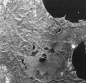
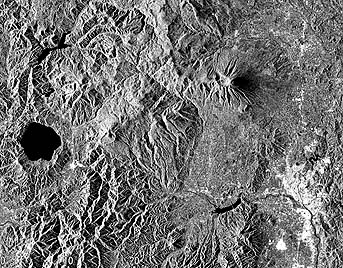
Next, we display a somewhat simpler, but still intriguing, geology, as the basaltic volcanic calderas, Volcan Alcedo (top) and Sierra Negra (left center) on Isabela Island, the largest of the Galapagos.
Try to locate the radar image in the following view (with north at the top) of much of the Galapagos group of islands made using the MISR sensor on Terra:
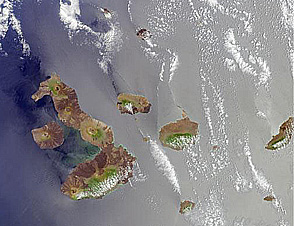
8-17: What is unusual about this image (clue: think of the volcanoes themselves)? ANSWER
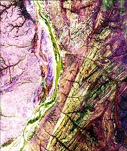
Below, the remarkable display of dendritic drainage in the SIR-A image of east-central Colombia results from uplands covered with grass that (because the blades are small) strongly reflects away the radar beam (thus dark), whereas the streams stand out as bright because their tree-lined channels produce double bounce reflections between the smooth water and tree trunks.
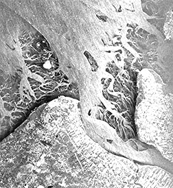
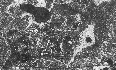
One property of radar pulses gave rise to an extraordinary image acquired from SIR-A in November, 1981. The color scene below is a Landsat subimage of the Selma Sand Sheet in the Sahara Desert within northwestern Sudan. Because dry sand has a low dielectric constant, radar waves penetrate these small particles several meters (about 10 ft). The inset radar strip trending northeast actually images bedrock at that general depth below the loose alluvial sand and gravel which acts as though almost invisible. It reveals a channeled subsurface topography, with valleys that correlate to specularly reflecting surfaces and uplands shown as brighter.
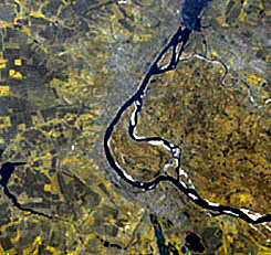
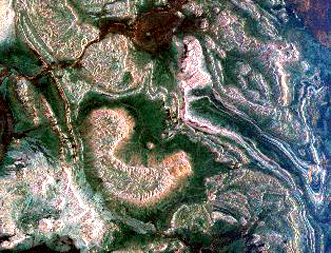
SIR-C radar continued this unmasking to the bedrock in Egypt because of this ability to penetrate the thin sand cover. This area of the Nile River shows to its left the underlying drainage pattern and to its right the rock units involved in a structurally complex geologic terrain:
Both Seasat and SIR-A were L-band radars. They differed mainly in altitude of operation and depression angle: Seasat at 790 km, angle = 67-73°; SIR-A at 250 km, angle = 37-43°; their spatial resolutions were similar. It is interesting to compare the same scene as witnessed by each system. Seasat had a near polar orbit, and SIR-A was confined (by Shuttle orbital configuration) to latitudes less than 38°. Look at this pair of views of the California coast and mountain ranges near Santa Barbara, with Seasat on top and SIR-A on bottom.
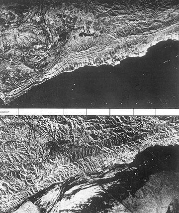
8-18: Compare the two radar system images, commenting especially on differences (and why)? ANSWER
SIR-B operated in 1984 over
eight days aboard another Shuttle mission. It differed from SIR-A in having a
variable look angle that ranged between 15° and 55°. Here is a SIR-B image L-band
image, taken at a 28° incidence angle of a forested area in northern Florida.
In April and October of
1994, a more versatile system flew twice on Shuttle missions. This system was
JPL's SIR-C, which had L- and C-band radars, each capable of HH, VV, HV, and
VH polarizations, and an X-band (X-SAR) instrument, supplied by German and Italian
organizations, that was in the VV mode. All of these radars had variable look
angles that imaged sidewards between 20° and 65°, producing resolutions between
10 and 25 m. One advantage of this multiband system was the ability to combine
different bands and polarizations into color composites. JPL's SIR-C Web Site
describes how to create composites. You can reach it by clicking here. It contains
a wealth of information and imagery, including our next set of images showing
the Kliuchevskoi Volcano in Kamchatka (Russian Siberia) as captured by SIR-C
in three polarization modes (L-band HH = blue; L-band HV = green; C-band HV
= red); on the left is a photo of the volcano taken at the same time by one
of the Shuttle astronauts.
Next, we show a multiband
(multifrequency) image of San Francisco, CA, made from L-bands HH (red) and
HV (green) and C-band HV (blue). It’s one of the most pleasing images
to the eye and it shows the city layout, which is a prime example of why so
many people want to live in the Bay Area after visiting it.
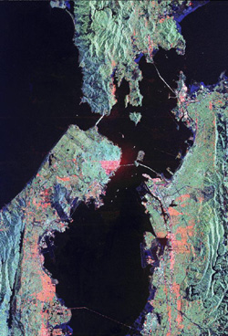
8-19: Name the bridges you can find in this image.
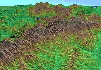
We can process SIR-C radar imagery taken on two dates (or with two antennas) using interferometric techniques that use signal phase differences to determine differences in distance to point targets to yield information on topographic variations. When combined with Digital Elevation Model (DEM) data (see page 11-5), single band or color composite radar images can show perspective views (page 11-8), as analglyphs (requiring stereo color glasses) (page 11-10), or even in simulated flyby videos. A perspective view of Death Valley and adjacent mountains made from SIR-C imagery is a good example.
The X-SAR instrument on SIR-C was supplied by Deutsches Zentrum fur Luft und Raumfahrt (DLR). This X-band (3 cm) radar operates in the VV mode. Here is an image of Hong Kong and adjacent mountains. Note the many ships in the waters near the city (Kowloon).
The next image was made from all three SIR-C bands: X-band = blue; C-band = green; L-band = red. The scene shows the city of Samarkind in Russia along the Volga River.
Another JPL radar system, the SRTM (Shuttle Radar Topography Mission) flown in the year 2000, will be discussed in a full page (11-10) in Section 11.
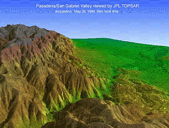
In conjunction with the SIR-C program, JPL flies an airborne system called AIRSAR/TOPSAR that includes an altimeter. One of its principal missions has been to simulate imagery similar to that produced from the TOPEX/Poseidon program. From this system, we present a multiband perspective view of the mountains just north of JPL's home in Pasadena, CA.
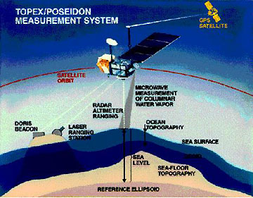
NASA/JPL, in conjunction
with the French Center for National Space Studies (CNES), has placed a radar
altimeter in space on the TOPEX/Poseidon
mission
launched on August 10,
1992. This JPL diagram summarizes the general mission configuration for TOPEX/Poseidon
(T/P):
Pointing straight down
(at nadir), this dual frequency (13.6 and 5.3 GHz) instrument transmits a
narrow beam of pulses whose variations in round-trip transit time represent
changes in altitude or (for oceans) wave heights along the 3-4 km swath line
(successive lines are spaced about 345 km [214 miles] apart at equatorial
crossings). The TOPEX altimeter can discriminate elevation differences of
13 cm. They operate TOPEX primarily for oceanographic studies, measuring the
effects of wind on waves, and the influence of currents and tides on marine
surfaces, and relating these to global climate change mechanisms. A second
French altimeter and a microwave radiometer (for atmospheric water measurements)
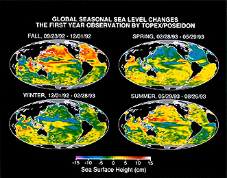
are among the six instruments onboard. The data gathered by TOPEX are not
normally displayed as images but are used to produce maps of regions or even
global hemispheres, as illustrated in the examples below (see page 14-12 for other
examples). The first image (map)
shows T/P sea surface height (SSH) variations (departures from a general mean
sea level) for 4 seasons in late 1992-1993.
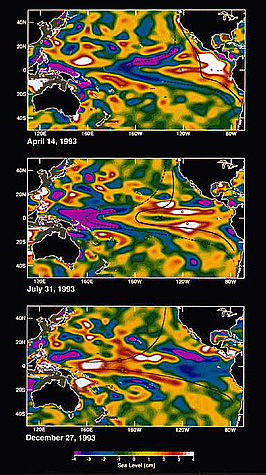
These three T/P maps
zero in on height variations in the mid-Pacific Ocean on three days in 1993:
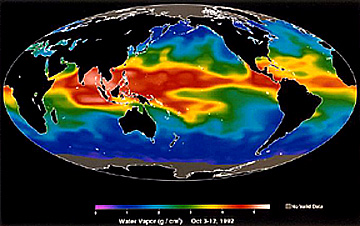
One of the instruments
on T/P is used to measure atmospheric water vapor - data used to make a needed
correction to improve SSH calculations. Here is a global map of water vapor
content.
One of the main tasks
assigned to T/P was determination of surface water temperatures using altimetric
data and other imputs. This has proved especially vital in monitoring the
variations of El Niño. This October 1997 shows a broad equatorial band of
very warm water (white) in the eastern Pacific adjacent to a cold band (purple)
in the western Pacific that corresponds to a near-maximum time of year for
that year's El Niño.
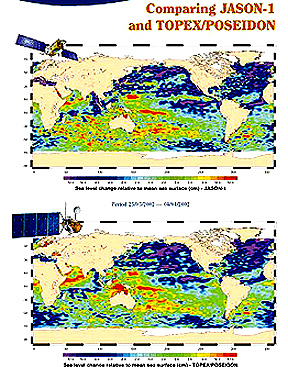
A T/P spacecraft is still operating. In late 2001, a follow-up NASA/CNES satellite,
called Jason-1, with greater surface height resolution, was launched (see page
14-12). As a preview,
compare these two images (Jason on top; T/P on bottom) taken over a short time
period in Fall of 1992.
International Radar Systems: Radarsat; ERS; ALMAZ; JERS;
As part of its ongoing program, the Canadian Space Agency on November 4, 1995, launched its first Radarsat-1 into a near-polar orbit at a height of 798 km (about 500 mi); this Web site also describes Radarsat2. This is a C-band SAR (5.3 GHz; wavelength 56 mm), whose look angle can range between 10° and 58° to provide swath widths between 35 and 500 km (22 to 311 mi), providing variable resolution centering around 25 m, but ranging from 9 to 100° as the look angle varies. The first image collected covered Cape Breton in northern Nova Scotia, shown heretofore on Page I-25.
This next Radarsat image covers a 70 km wide area in the northern part of Honshu, the main island of Japan. Note Lake Tazawako, the volcano (Mt. Iwati) and the small city of Morioka (white patch near lower right).
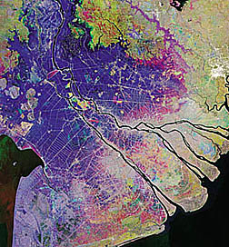
Single band images can be colorized (assigned colors to different gray levels) to help bring out features whose radar returns vary; to some degree in such an image, specific colors may actually relate to separable classes of features. This radar image of the Mekong Delta in South Vietnam shows some color/feature correlation:
As with most of the other
systems previously described, users can convert images from Radarsat using separate
topographic data into perspective views. This next image was made from a radar
scan over the Tuzla district in Bosnia-Herzogovina, in the Balkans.
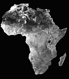
Making mosaics of radar
images is a fairly easy job since the variability of lighting from different
Sun angles as occurs during the changing seasons, which characterizes systems
like Landsat and SPOT, is not a factor with radar (although this constancy
of radar illumination must be fixed by the same Look Angles and proper overlap
conditions). Sixteen hundred Radarsat images have been combined to make a
continental-scale mosaic of the African continent:
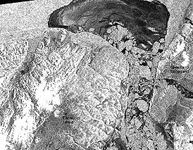
One of the prime tasks
for which Radarsat was flown by the Canadians is to monitor sea ice in their
northern (Arctic) waters. The distribution and characteristics of sea ice
affect both the (limited) operations of ocean shipping and the extent to which
open waters will affect climate (and vice versa). Here is an image of sea
ice around Ellesmere Island west of northern Greenland:
Different types of ice
cover can be distinguished when on the ice, or looking from a ship or an airplane.
Classes can be set up, based on whether the ice is smooth (fast ice), or deformed
in differnt ways and degrees. A classification (right image below) of a small
area of Canadian Arctic ocean (left image) met with considerable success.
In the legend on the
right, blue indicates open water, yellow shows fast ice, green is assigned
to somewhat deformed ice, and red denotes notably deformed ice. The Europeans and Japanese
have now flown radars on unmanned space platforms. Some information about
the European mission is available in JPL's Radar Home Page under the topic
Earth Resources Satellites
(ERS). The European Space Agency (ESA) launched ERS-1,
with a complement of sensors, in July, 1991, at a nominal altitude of 800
km (500 mi). Along with a radar scatterometer, it carried a C-band, VV SAR
with a fixed look angle extending from 20° to 26°. This next scene shows a
color composite, made from multidate images, of the farmlands (including vineyards)
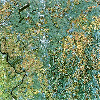
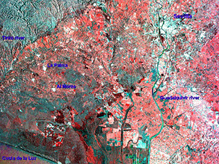
along the Rhine near the city of Darmstadt. A nearly identical SAR
was on ERS-2, which launched in April, 1995. Users can construct innovative
color composites from the single band, single polarization radar by using
images from different dates. We show here an example of this process: a multi-date
image of Sevilla, Spain, in which an ERS-1 image on Nov. 3, 1993, is assigned
to red; an ERS-1 image on June 9, 1995, is green, and an ERS-2 image on June
10, 1995, is blue. The city of Seville appears in a cyan tone in the upper
right, as does the Sierra de Aracena in the upper left, and agricultural fields
(bright, but barren) show as red in the rest of the image.
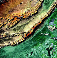
One of the most impressive
radar products from ERS-2 shows tilted beds in western China:
The Russian Space program,
since it entered the commercial marketplace, has released (through SovInformSputnik)
some of the radar images acquired by its ALMAZ radar satellites. An example
shows the mouth of the Elbe River along the northern Germany coastline:
JERS-1, launched to a
570 km (354 mi) orbit on February 11, 1992, by the Japanese National Space Agency,
contained a seven band optical sensor and a SAR. The latter was L-band with
HH polarization. It had a fixed look angle view between 32° and 38°, yielding
a swath width of 75 km and a mean resolution of 18 m. One of its first images
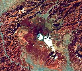
covered Mt. Fuji, a stratocone volcano west of Tokyo, as shown here. 8-20: Here
is a puzzler. I have determined that the very bright patches are the small
city of Fujiyoshida. How did I do that (remember to rely on your World Atlas).ANSWER By way of comparison,
here is a false color composite of Fujiyama made by the Japanese MOS-1 (Marine
Observation Satellite; see page
14-12).
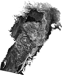
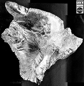
A spectacular JERS radar
image is this mosaic scene of the Big Island of Hawaii:
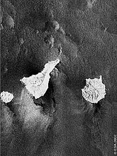
The latest entry into
commercially available radar imagery is the ASAR (Advanced SAR) sensor onboard
ESA's Envisat (see page
16-10a for details. Two tasks of that instrument are 1) to observe sea
state, and 2) to monitor high latitude ice conditions. The first is exemplified
by this view of the Atlantic Ocean waters around the Canary Islands:
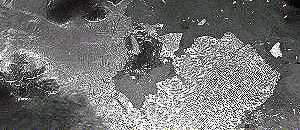
The second is illustrated
by this image of ice, open water, and land in the Arctic:
And, as we have seen
before in the Overview, the C-Band ASAR is capable of producing colorized
images, such as this view of part of the Volga River in Russia, using different
viewing modes; the image appears flat (no relief) because this is part of
the steppe plains of western Russia and the Ukraine which has little variation
in elevations - hence no conspicuous hilly irregularities.
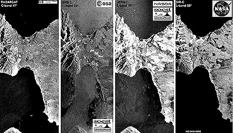
Each radar satellite
tends to show a given scene in its own particular way, depending on band(s)
used, Look Angle, polarization and other factors. Compare this small part
of the island of Maui in the Hawaiian Islands as seen by (left to right) Radarsat,
ERS-2, JERS-1, and SIR-C.
The advent of radar systems
into space, following their effective demilitarization worldwide, provides
the remote sensing communities with a powerful source of environmental and
mapping data that are obtainable over any part of the Earth. With altimeter
or interferometric processing, radar presents a new capability to generate
topographic maps for parts of the global land surface, viewable from near-polar
orbits. Information on several aspects of ocean surface states is also a valuable
payoff. The prospects of using multi-frequency, multi-polarization beams to
obtain distinctive radar signatures offers another means to identify materials
that are separable on the basis of dielectric constants, surficial roughness,
and other properties.