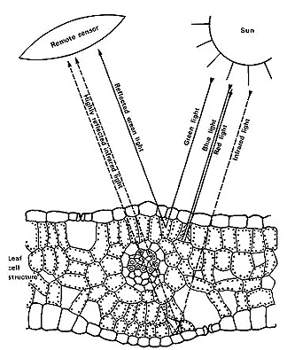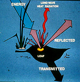
Now, consider this diagram
which traces the influence of green leafy material on incoming and reflected radiation.
Absorption centered at
about 0.65 µm (visible red) by chlorophyll pigment in green-leaf chloroplasts
that reside in the outer or Palisade leaf, and to a similar extent in the blue,
removes these colors from white light, leaving the predominant but diminished
reflectance for visible wavelengths concentrated in the green. Thus, most vegetation
has a green-leafy color. There is also strong reflectance between 0.7 and 1.0
µm (near IR) in the spongy mesophyll cells located in the interior or back of
a leaf, within which light reflects mainly at cell wall/air space interfaces,
much of which emerges as strong reflection rays. The intensity of this reflectance
is commonly greater (higher percentage) than from most inorganic materials,
so vegetation appears bright in the near-IR wavelengths. These properties of
vegetation account for their tonal signatures on multispectral images: darker
tones in the blue and, especially red, bands, somewhat lighter in the green
band, and notably light in the near-IR bands (maximum in Landsat's Multispectral
Scanner Bands 6 and 7 and Thematic Mapper Band 4 and SPOT's Band 3).
Identifying vegetation in
remote-sensing images depends on several plant characteristics. For instance,
in general, deciduous leaves tend to be more reflective than evergreen needles.
Thus, in infrared color composites, the red colors associated with those bands
in the 0.7 - 1.1 µm interval are normally richer in hue and brighter from tree
leaves than from pine needles.
These spectral variations
facilitate fairly precise detecting, identifying and monitoring of vegetation
on land surfaces and, in some instances, within the oceans and other water bodies.
Thus, we can continually assess changes in forests, grasslands and range, shrublands,
crops and orchards, and marine plankton, often at quantitative levels. Because
vegetation is the dominant component in most ecosystems, we can use remote sensing
from air and space to routinely gather valuable information for characterizing
and managing of these organic systems.
One of the most successful
applications of multispectral space imagery is monitoring the state of the world's
agricultural production. This application includes identifying and differentiating
most of the major crop types: wheat, barley, millet, oats, corn, soybeans, rice,
and others.
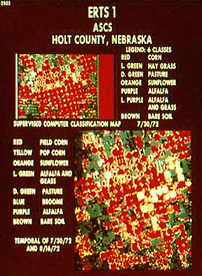
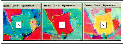
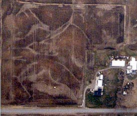
This capability was convincingly
demonstrated by an early ERTS-1 classification of several crop types being grown
in Holt County, Nebraska. This pair of image subsets, obtained just weeks after
launch, indicates what crops were successfully differentiated; the lower image
shows the improvement in distinguishing these types by using data from two different
dates of image acquisition:
Perhaps this is a good
point in the discussion to introduce the appearance of large area croplands
as they appear in Landsat. We will illustrate with imagery that cover the two
major crop growing areas of the United States.
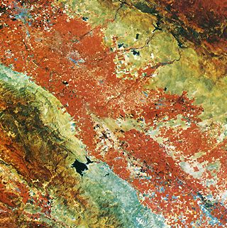
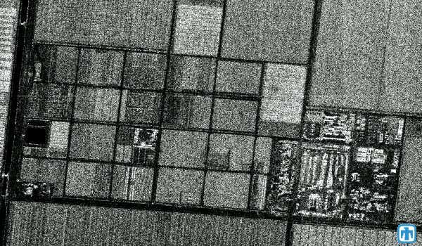
The first is part of the Great
or Central Valley of California, specifically the San Joaquin Valley. Agricultural
here is primarily associated with such cash crops as barley, alfalfa, sugar beets,
beans, tomatoes, cotton, grapes, and peach and walnut trees. In July of 1972 most
of these fields are nearing full growth. Irrigation from the Sierra Nevada, whose
foothills are in the upper right compensates for the sparsity or rain in summer
months. The eastern Coast Ranges appear at the lower left. The yellow-brown and
blue areas flanking the Valley crops are grasslands and chapparal best suited
for cattle grazing. The blue areas within the croplands (near the top) are the
cities of Stockton and Modesto.
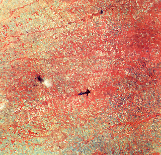
The second Landsat image
is in the Wheat Belt of the Great Plains. The image below is of western Kansas
in late August. Most of the scene consists of small farms, many of section size
(1 square mile). The principal crop is winter wheat which is normally harvested
by June. Spring wheat is then planted, along with sorghum, barley, and alfalfa.
This scene is transitional, with nearly all of the right side being heavily
planted, but the left side (the High Plains, at higher elevations) contains
some unplanted farms and barren land, some used for grazing.
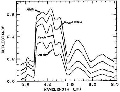
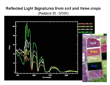
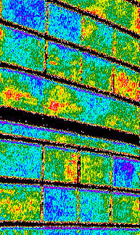
Many factors combine to cause
small to large differences in spectral signatures for the varieties of crops cultivated
by man. Generally, we must determine the signature for each crop in a region from
representative samples at specific times. However, some crop types have quite
similar spectral responses at equivalent growth stages. The differences between
crop (plant) types can be fairly large in the Near-Infrared, as shown in these
spectral curves (in which other variables such as soil type, ground moisture,
etc. are in effect held constant).
3-1:
Drawing on your experience and common sense, make (or
think) a list of the factors that will affect the spectral signatures of field
crops. ANSWER
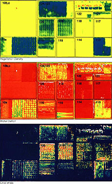
Through remote sensing it
is possible to quantify on a global scale the total acreage dedicated to these
and other crops at any time. Of greater import, is accurately (best case 90%)
estimating the expected yields (production in bushels or other units) of each
crop, locally, regionally or globally. We do this by first computing the areas
dedicated to each crop, and then incorporating reliable yield assessments per
unit area, which agronomists can measure at representative ground-truth sites
(or in the U.S., county farm agents obtain routinely from the farmers themselves).
Reliability is enhanced by using the repeat coverage of the croplands afforded
by the cyclical satellite orbits assuming, of course, cloud cover is sparse enough
to foster several good looks during the growing season. Usually, the yield estimates
obtained from satellite data are more comprehensive and earlier (often by weeks)
than determined conventionally as harvesting approaches. Information about soil
moisture content, often critical to good production, can be qualitatively (and
under favorable conditions, quantitatively) appraised with certain satellite observations.
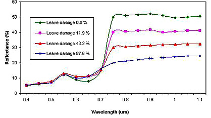
Under suitable circumstances,
it is feasible to detect crop stress generally from moisture deficiency or disease
and pests, and sometimes suggest treatment before the farmers become aware of
problems. Stress is indicated by progressive decrease in Near-IR reflectance,
as evidenced in this set of field spectral measurements of leaves taken from soybean
plants as these underwent increasing stress that causes loss of water and breakdown
of cell walls.
Differences in vegetation
vigor, resulting from variable stress, are especially evident when Near Infrared
imagery or data are used. In this aerial photo made with Color IR film shows
healthy vegetation in red, and "sick" (stressed) vegetation in blue to yellow-white:
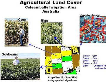
For identifying crops, two
important parameters we use are the size and shape of the crop type ( e.g. soybeans
have spread out leaf clumps; corn has tall stalks with long, narrow leaves and
thin, tassle-topped stems; and wheat [in the cereal grass family] has long thin
central stems with a few small, bent leaves on short branches, all topped by a
head containing the kernels from which flour is made). Other considerations are
the surface area of individual leaves, the plant height and amount of shadow it
casts, and the spacing or other planting geometries of row crops (the normal arrangement
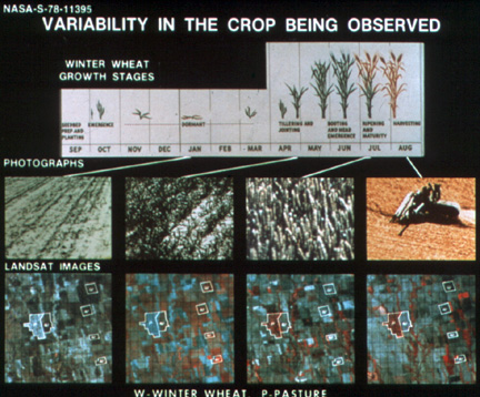
of legumes, feed crops, and fruit orchards). The stage of growth (degree of crop
maturity) is also a factor. For example during its development wheat, passes through
several distinct steps such as, developing its kernel-bearing head, and changing
from shades of green to golden-brown (see below).
Another related parameter
is Leaf Area Index (LAI), defined as the ratio of one-half the total area of leaves
(the other half is the underside) in vegetation to the total surface area containing
that vegetation. If all the leaves were removed from a tree canopy and laid on
the ground, their combined areas relative to the ground area projected beneath
the canopy would be some number greater than 1 but usually less than 10. As a
tree, for example, fully leaves, it will produce some LAI value that is dependent
on leaf size and shape, the number of limbs, and other factors. The LAI is related
to the the total biomass (amount of vegetative matter [live and dead] per unit
area, usually measured in units of tons or kilograms per hectare [2.47 acres])
in the plant and to various measures of Vegetation Index (see below). Estimates
of biomass can be carried out with variable reliability using remote sensing inputs,
provided there is good supporting field data and the quantitative (mathematical)
models are efficient. Both LAI and NDVI (page 3-4) are used in the
calculations.
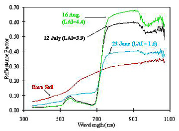
In principal, actual LAI
must be determined on site directly by stripping off all leaves, but in practice
it can be estimated by statistical sampling or by measuring some property such
as reflectance. Thus, remote sensing can determine an LAI estimate if the reflectances
are matched with appropriate field or ground truth. For remotely sensed crops,
LAI is influenced by the amount of reflecting soil between plant (thus looking
straight down will see both corn and soil but at maturity a cornfield seems
closely spaced when viewed from the side). For the spectral signatures shown
below, the Near IR reflectances will increase with LAI.
This change in appearance
and extent of surface area coverage over time is the hallmark of vegetation as
compared with most other categories of ground features (especially those not weather-related).
Crops in particular show strong changes in the course of a growing season, as
illustrated here for these three stages - bare soil in field; full growth; fall
senescence:
3-2:
How would non-growing or dead vegetation (such as crops
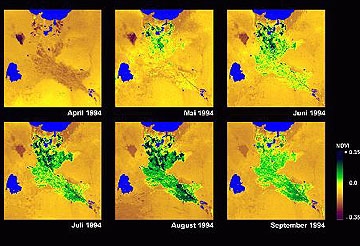
in senescence) be detected by Landsat? ANSWER The study of vegetation
dynamics in terms of climatically-driven changes that take place over a growing
season is called phenology. A good example of how repetitive satellite
observations can provide updated information on the phenological history of
natural vegetation and crops during a single cycle of Spring-Summer growth is
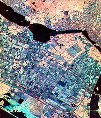
this sequence of AVHRR images of the Amu-Dar'ja Delta just south of the Aral
Sea in Ujbekistan (south-central Asia).The amount of vegetation present in the
delta (a major farming district for this region) is expressed as the NDVI, an
index defined on page
3-4. The Aral Sea - a large inland lake - is now rapidly drying up (see
page page 14-15).
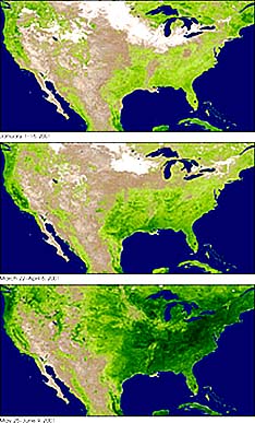
More generally, seasonal
change appears each year with the "greening" that comes with the advent of Spring
into Summer as both trees and grasses commence their annual growth. The leafing
of trees in particular results in whole regions becoming dominated by active
vegetation that is evident when rendered in a multispectral image in green tones.
The MODIS sensor on Terra has several vegetation-sensitive bands used to calculate
a variation of the NDVI called the Enhanced Vegetation Index (EVI). This trio
of images (dates in the caption) shows the spread of growing natural vegetation
across the U.S.
To emphasize the variability
of the spectral response of crops over time, we show these phenological stages
for wheat in this sequential illustration: