This and the next four pages deal with the process of classifying multispectral images into patterns of varying gray or assigned colors that represent either clusters of statistically different sets of multiband data (radiances expressed by their DN values), some of which can be correlated with separable classes/features/materials (Unsupervised Classification), or numerical discriminators composed of these sets of data that have been grouped and specified by associating each with a particular class, etc. whose identity is known independently and which has representative areas (training sites) within the image where that class is located (Supervised Classification). The principles involved in classification, mentioned briefly in the Introduction, are explored in more detail. This page also describes the approach to unsupervised classification and gives examples; it is pointed out that many of the areas classified in the image by their cluster values may or may not relate to real classes (misclassification is a common problem).

Now, at last we approach the finale of this Tutorial section during which we demonstrate two of the common methods for identifying and classifying features in images: Unsupervised and Supervised Classification. Closely related to Classification is the approach called Pattern Recognition. A helpful Internet site on classification procedures can be read at the outset.

Before starting, it is well to review several basic principles, considered earlier in the Introduction, with the aid of this diagram:

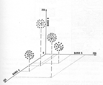
In the upper left are plotted spectral signatures for three general classes: Vegetation; Soil; Water. The relative spectral responses (reflectances in this spectral interval), in terms of some unit, e.g., reflected energy in appropriate units or percent (as a ratio of reflected to incident radiation, times 100), have been sampled at three wavelengths. (The response values are normally converted [either at the time of acquisition on the ground or aircraft or spacecraft] to a digital format, the DNs or Digital Numbers cited before, commonly subdivided into units from 0 to 255 [2⁸]).

For this specific signature set, the values at any two of these wavelengths are plotted on the upper right. It is evident that there is considerable separation of the resulting value points in this two-dimensional diagram. In reality, when each class is considered in terms of geographic distribution and/or specific individual types (such as soybeans versus wheat in the Vegetation category), as well as other factors, there will be usually notable variation in one or both chosen wavelengths being sampled. The result is a spread of points in the two-dimensional diagram (known as a scatter diagram), as seen in the lower left. For any two classes this scattering of value points may or may not overlap. In the case shown, which treats three types of vegetation (crops), they don't. The collection of plotted values (points) associated with each class is known as a cluster. It is possible, using statistics that calculate means, standard deviations, and certain probability functions, to draw boundaries between clusters, such that arbitrarily every point plotted in the spectral response space on each side of a boundary will automatically belong the class or type within that space. This is shown in the lower right diagram, along with a single point "w" which is an unknown object or pixel (at some specific location) whose identity is being sought. In this example, w plots just in the soybean space.

Thus, the principle of classification (by computer image-processing) boils down to this: Any individual pixel or spatially grouped sets of pixels representing some feature, class, or material is characterized by a (generally small) range of DNs for each band monitored by the remote sensor. The DN values (determined by the radiance averaged over each spectral interval) are considered to be clustered sets of data in 2-, 3-, and higher dimensional plotting space. These are analyzed statistically to determine their degree of uniqueness in this spectral response space and some mathematical function(s) is/are chosen to discriminate the resulting clusters.

Two methods of classification are commonly used: Unsupervised and Supervised. The logic or steps involved can be grasped from these flow diagrams:

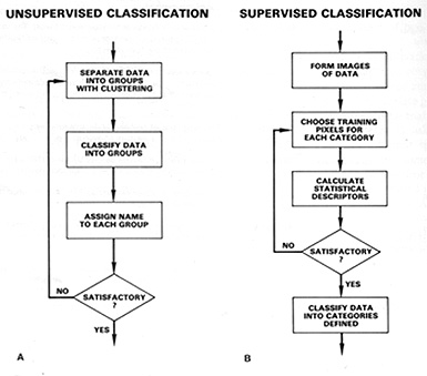
In unsupervised classification any individual pixel is compared to each discrete cluster to see which one it is closest to. A map of all pixels in the image, classified as to which cluster each pixel is most likely to belong, is produced (in black and white or more commonly in colors assigned to each cluster. This then must be interpreted by the user as to what the color patterns may mean in terms of classes, etc. that are actually present in the real world scene; this requires some knowledge of the scene's feature/class/material content from general experience or personal familiarity with the area imaged. In supervised classification the interpreter knows beforehand what classes, etc. are present and where each is in one or more locations within the scene. These are located on the image, areas containing examples of the class are circumscribed (making them training sites), and the statistical analysis is performed on the multiband data for each such class. Instead of clusters then, one has class groupings with appropriate discriminant functions that distinguish each (it is possible that more than one class will have similar spectral values but unlikely when more than 3 bands are used because different classes/materials seldom have similar responses over a wide range of wavelengths). All pixels in the image lying outside training sites are then compared with the class discriminants, with each being assigned to the class it is closest to - this makes a map of established classes (with a few pixels usually remaining unknown) which can be reasonably accurate (but some classes present may not have been set up; or some pixels are misclassified.

Both modes of classification will be considered in more detail and examples given here and on the next 4 pages.

In an unsupervised classification, the objective is to group multiband spectral response patterns into clusters that are statistically separable. Thus, a small range of digital numbers (DNs) for, say 3 bands, can establish one cluster that is set apart from a specified range combination for another cluster (and so forth). Separation will depend on the parameters we choose to differentiate. We can visualize this process with the aid of this diagram, taken from Sabins, "Remote Sensing: Principles and Interpretation." 2nd Edition, for four classes: A = Agriculture; D= Desert; M = Mountains; W = Water.

From F.F. Sabins, Jr., "Remote Sensing: Principles and Interpretation." 2nd Ed., © 1987. Reproduced by permission of W.H. Freeman & Co., New York City.

We can modify these clusters, so that their total number can vary arbitrarily. When we do the separations on a computer, each pixel in an image is assigned to one of the clusters as being most similar to it in DN combination value. Generally, in an area within an image, multiple pixels in the same cluster correspond to some (initially unknown) ground feature or class so that patterns of gray levels result in a new image depicting the spatial distribution of the clusters. These levels can then be assigned colors to produce a cluster map. The trick then becomes one of trying to relate the different clusters to meaningful ground categories. We do this by either being adequately familiar with the major classes expected in the scene, or, where feasible, by visiting the scene (ground truthing) and visually correlating map patterns to their ground counterparts. Since the classes are not selected beforehand, this latter method is called Unsupervised Classification.

The IDRISI image processing program employs a simplified approach to Unsupervised Classification. Input data consist of the DN values of the registered pixels for the 3 bands used to make any of the color composites. Algorithms calculate the cluster values from these bands. It automatically determines the maximum number of clusters by the parameters selected in the processing. This process typically has the effect of producing so many clusters that the resulting classified image becomes too cluttered and, thus, more difficult to interpret in terms of assigned classes. To improve the interpretability, we first tested a simplified output and thereafter limited the number of classes displayed to 15 (reduced from 28 in the final cluster tabulation).

1-20: What's to be done if one uses more than three bands to make an Unsupervised Classification? ANSWER

The first Unsupervised Classification operates on the color composite made from Bands 2, 3, and 4. Examine the resulting image when just 6 clusters are specified.

The light buff colors associate with the marine waters but are also found in the mountains where shadows are evident in the individual band and color composite images. Red occurs where there is some heavy vegetation. Dark olive is found almost exclusively in the ocean against the beach. The orange, green, and blue colors have less discrete associations.

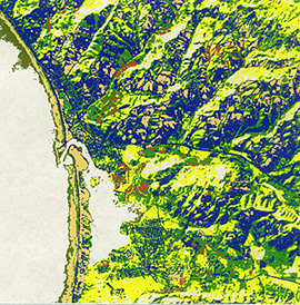
We next display a more sophisticated version, again using Bands 2, 3, and 4, in which 15 clusters are set up; a different color scheme is chosen.

Try to make some sense of the color patterns as indicators of the ground classes you know from previous paragraphs. A conclusion that you may reach is that some of the patterns do well in singling out some of the features in parts of the Morro Bay subscene. But, many individual areas represented by clusters do not appear to correlate well with what you thought was there. Unfortunately, what is happening is a rather artificial subdivision of spectral responses from small segments of the surface. In some instances, we see simply the effect of slight variations in surface orientation that changes the reflectance's or perhaps the influence of what we said in the Overview was "mixed pixels". When we try another composite, Bands 4, 7, and 1, the new resulting classification has most of the same problems as the first, although sediment variation in the ocean is better discriminated. One reason why both 15 cluster classifications don't grab one's attention is that the colors automatically assigned to each cluster are not as distinctly different (instead, some similar shades) as might be optimum.

1-21: Critique these two Unsupervised Classifications. What is shown well; poorly? Do you find it very helpful in pinpointing potential classes to be identified and then used in carrying out a supervised classification? ANSWER

We conclude that Unsupervised Classification is too much of a generalization and that the clusters only roughly match some of the actual classes. Its value is mainly as a guide to the spectral content of a scene to aid in making a preliminary interpretation prior to conducting the much more powerful supervised classification procedures.