As applied to star analysis, four kinds of spectral data are relevant: 1) Continuous spectra; 2) Emission Line spectra; 3) Absorption Line spectra; and 4) Blackbody radiation spectra. The first three are illustrated here:

A Continuum Spectrum,
particularly as it applies to the UV, Visible, and Near IR segments of the ElectroMagnetic
Spectrum, is that produced by white light, i.e., all wavelengths (all colors in
the Visible) in this region are present in essentially equal proportions. An Emission
Line Spectrum results when photons of narrow, specific wavelengths are emitted
during excitation of the elements present in an emitting body; each (colored)
line is diagnostic (identifies) some particular element. An Absorption Line
Spectrum occurs when the emitted radiation from a hot body passes through
cooler gases containing the same elements as those responsible for the emitted
photons which interact (by absorption processes) and are removed from the continuum
(as shown by black lines). A Blackbody Spectrum, discussed in detail on page 9-1 and 9-2, is a continuum
spectrum that is associated with the thermal state of an emitting body considered
to be a perfect radiator, especially one heated to incandescence, in which
its spectral curve peaks at some wavelength which varies systematically with temperature.
This figure should remind you of the information presented on page 9-2 dealing
with Wien's Displacement Law.
Now, in more detail: Each
element has a series of spectral lines that are diagnostic, being found in fixed
locations in a spread of the spectrum as determined by the wavelengths of emitted
radiation resulting from excitation of electrons into higher energy levels (recall
the formula: ΔE = hν). Emission lines relate to light (including UV
and IR) radiation passing unimpeded from the source. But, starlight normally
must pass through the star's atmosphere; if the outer gases contain the same
elements as those from its surface, the emitted radiation will be absorbed at
the characteristic wavelengths, giving rised to absorption spectra. The image
below is the spectrum for our Sun, with the dark absorption (Frauenhofer) lines
correlating mostly with hydrogen and helium:
Since hydrogen is by far
the most common element in the Universe, comments on its spectra are in order;
the principles involved in the generation of hydrogen's spectral lines apply
to all other elements. Radiation from excited hydrogen is detectable over most
of the EM spectral range, but important and diagnostic radiation at specific
wavelengths used by astronomers extend from the Ultraviolet through much of
the Infrared Range. Emitted radiation results when the single electron in the
neutral hydrogen atom is excited by various forms of energy (e.g., heat, electrical
current, particle bombardment) such that the electron is displaced from its
ground state to one or more of the various energy levels associated with the
possible orbital levels surrounding the nucleus. These are energy levels that
are discrete (specific values) in terms of the quantum states possible when
excitation has occurred. These levels are, by convention, represented by the
letter "N" and are expressed as integers from 1 through 2, 3, 4, 5,6, .....
infinity. In the ground state, the electron resides in level 1 (or shell, as
is often depicted in the Bohr atom model). When excitation energy is provided,
the electron can "jump" to higher (quantized) levels, as, for example from N
= 1 to N = 3. That energy is calculated by the familiar Planck equation: ΔE
= hν, where the ΔE is the energy required to move to a specific
level, say from 1 to 3, shown as E3 - E1, h is the Planck
constant, and ν is the frequency (its reciprocal is the wavelength &lamda;.
In the higher energy states (multiples of N greater than 1), the electron may
remain for a time in a metastable mode but for most of the transitions the electron
almost instantly returns to a lower energy state (either to the ground state
N = 1 or to one of the lower levels of N than the level first reached by the
electron. When the return occurs, the excitation energy is given off as photons
whose specific frequency (or wavelength equivalent) is determined by δE.
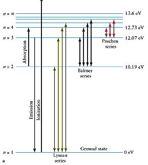
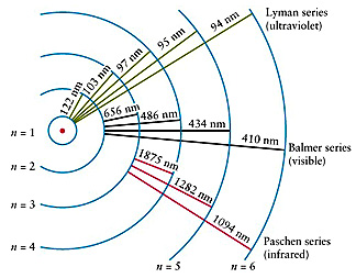
Examine this diagram:
For the Lyman series (of
transitions expressed as spectral lines of very precise wavelengths), the electrons
will move to different N levels and then revert to the N = 1 state. For the
Balmer series, the reverted level is N = 2; the Paschen series, N = 3. To illustrate
with specific values, consider the Balmer series, in which the four principal
lines, designated as Hα, Hβ, Hγ,
and Hδ, require (in the same sequence) energies (hν)of
3.02 x 10⁻¹⁹ , 4.07 x 10⁻¹⁹, 4.57 x 10⁻¹⁹,
and 4.84 x 10⁻¹⁹ Joules (J), and give off photons whose wavelengths
(state here in nanometers [µm x 1000) are 656.3, 486.1, 434.0, and 410.2 nm
respectively. The Balmer wavelengths are all in the Visible region of the spectrum.
The Lyman series occurs in the Ultraviolet and the Paschen series in the near
Infrared segments of the EM spectrum. There are other series (not named) elsewhere
in the EM spectrum. Now, look at this next diagram - a variant of the one above
but with added information:
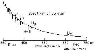
All of these lines are
found in solar spectra. A spectral curve (the spectrum as plotted on a strip
chart recorder) from an O-type (very hot) star produces absorption spikes for
the Balmer series in the Visible; it looks like this:
As was first treated, on
page 20-5, letters in the sequence O-B-A-F-G-K-M refer to spectral classes of
stars; the sequence is also an observed temperature indicator with each letter
denoting a range of temperatures, with O hottest (greater than 10000°K) and
M coolest (less than 3000°K), Typical spectra for the different classes of stars
on the Main Sequence will include lines for hydrogen, helium, and other elements,
shown as follows:
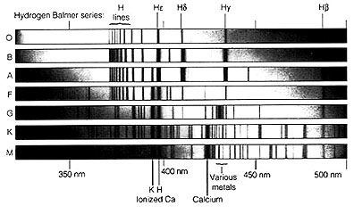
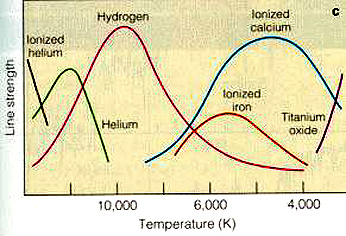
The following are principal
spectral lines within the Visible spectrum representing the different stellar
classes, with surface temperatures plotted on the ordinate:
This next diagram helps
to categorize the spectral classes O through M, in which for each class a range
of spectral lines of certain individual or several elements are diagnostic and
may predominate. Thus an A star shows strong hydrogen lines with some neutral
helium and ionized metals contributing their lines whereas a K star spectrum
is predominantly that of calcium and excited neutral metals.
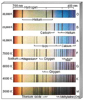
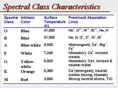
This can be restated in
the following chart that names the star class, its intrinsic surface color,
a characteristic surface temperature, and the principal diagnostic spectral
lines.
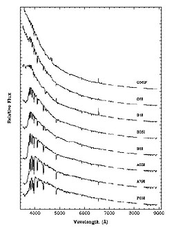
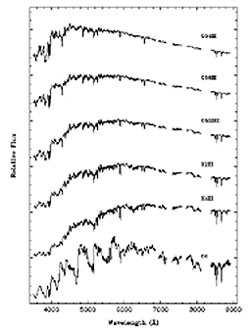
The stars off the Main
Sequence will, of course, show different spectral patterns depending on their
compositions. Below are two sets of spectral curves, with individual lines noted
as downward spikes in part of a Blackbody spectrum (see page
9-2) in the spectral range from 4000-9000 nm (0.4-0.9 µm) range. The left
set covers spectra from Blue Giants; the right from Red Giants. The shift in
peaks is a function of temperature. The left group is dominated by hydrogen
lines; in the right group some lines include calcium.
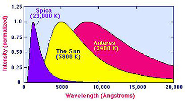
These plots suggest that
the shape of the overall Blackbody spectrum will vary as a function of temperature.
This is apparent in these generalized Blackbody spectral curves for a very hot
star (Spica), the Sun, and the cool star Antares:
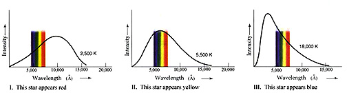
The general Blackbody curve
as it shifts with temperature also aids in showing how individual stars display
the colors astronomers assign to them. Consider this illustration:
The left curve, for a cool
star, shows that the part of the highest part on the curve intersected by the
color spread in the Visible spectrum is associated with red, hence such stars
are defined colorwise by Red. In the middle curve, the high point on the curve
is straddled by yellow; a Sunlike star then is Yellow (or Orange). The right
curve, for a hot star, has the visible blue at a higher intensity than green
or red and hence defines a Blue star (actually, as it appears, such a star is
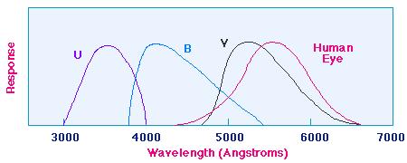
a bright bluish-white). This suggests that color
can be used in the Letter classification. Astronomers have developed a Color
Index system of relating stars to their surface temperatures. A given star is
observed through a telescope at three different wavelength ranges, one (U) centering
in part of the Ultraviolet, a second (B) in the Blue, and a third (V) in the
longer wavelength part of the Visible. The starlight passes through three filters,
as shown:
The intensity of light
received through each filter can either be expressed in flux terminology or,
more commonly, converted into an apparent magnitude value "m" appropriate to
the spectral range (e.g., mB). In turn, this magnitude must then
be converted an absolute magnitude M and then corrected for atmospheric effect
to produce what is termed a bolometric magnitude Mbol. This is necessary
so that all stars are compared in brightness at the same fixed distance. A Color
Index value in the UBV system is then calculated as B - V (and/or U - B), by
mathematically subtracting the bolometric magnitudes, as for instance, mB
- MV
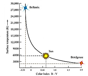
The Index can have positive
or negative values. Hotter stars have C.I.'s that are negative or slightly positive;
as magnitudes decrease with lower temperatures the Index becomes more positive.
The Sun's B - V Color Index is +0.62. In the third illustration above the star
Spica has a B - V of -0.22 and Betelgeuse a value of +1.85. A hotter star than
the Sun would have a smaller +C.I. or, with increasing temperature, values that
become negative.
Now, with this background,
let us turn our attention to how elements of atomic number above 4 have been produced
by stellar processes. In the first half billion or so years after the Big Bang,
the elemental chemistry of the Universe was quite simple. Hydrogen and helium
dominated, with very small amounts of several slightly heavier elements produced
during the early days. As galaxies began to organize from clots of slightly denser
hydrogen, the first stars formed. At that time many (most) were very massive O
and B types. These have very short lifetimes, sometimes burning their fuel in
a few million years. Their fate is to explode as supernovae, as described on page
20-6. Even smaller stars that work through the Red Giant stage have, or will,
eventually cast off a considerable amount of their elemental constituents enroute
to becoming White Dwarfs.
Stars, particularly the massive
ones mentioned above, are the furnaces in which the elements beyond H, He, and
some Li are created (stellar nucleosynthesis) by successive steps in nuclear
fusion in which more and more protons and neutrons are joined into stable to unstable
nuclei. The development of shells of elements with mass numbers greater than 2
is shown for two common cases: 1) a star of overall mass and size similar to the
Sun, and 2) A star with about 100 solar masses (not scaled; the stars are not
the same size).
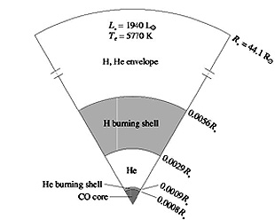
Stars with solar masses between
1 and 10 (those that follow the asymptotic giant branch [AGB] described on page 20-5) tend to burn their
helium into carbon and some oxygen but do not form elements of higher atomic numbers.
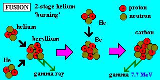
Much of the burning involves fusion of three helium atoms according to this sequence:
The red giant that results
shows the distribution of elements after fusion has produced these element shells;
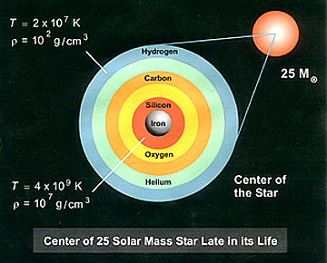
A typical, but somewhat generalized
sequence of nucleosynthesis of elements of atomic number higher than oxygen (>8)
is depicted in the figure below for a star composed initially of 25 solar masses
(MO) of hydrogen, but now is approaching (there is some hydrogen left)
its final stage of evolution (before exploding as a supernova_ in which the star
consists of a sequence of elements formed progressively with depth as it heated
up and contracted. Stars with greater than 10 solar masses will proceed to the
iron core stage; a Sun-sized star reaches only the carbon core stage.
As a massive hydrogen-rich
star contracts and experiences greater pressures, helium is the first nuclear
product within its core region. The energy released from fusion, along with continuing
densification, yields higher temperatures (1-2 x 10⁸ K) that transmute
this innermost helium into carbon (by fusion of three helium nuclei) while producing
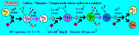
new helium at the next outer shell, but with hydrogen still dominant. This so-called
CNO (Carbon-Nitrogen-Oxygen) burning cycle is illustrated here:
Once carbon is formed in abundance,
this helium is generated as an end product of the CNO cycle. In this, some C12
reacts with protons to generate, in successive steps, N13, N14,
N15 and then O15. After this last step, that unstable oxygen
isotope can fuse with a proton and then decay by fission, thereby releasing an
alpha particle (He4, stripped of its electrons) causing the reversion
to C12.
Ever greater contraction,
with concomitant temperatures reaching > 5 x 10⁸ K for elements
like sodium and magnesium, 1 x 10⁹ K for oxygen, and approaching
3 x 10⁹ K for nickel, cobalt, and iron, can progressively generate
the elements listed in the figure up to iron (plus others of lesser atomic numbers)
in amounts proportional to the comparative solar masses indicated. Thus, a star
massive enough to ultimately achieve an iron core also contains elements of
lower atomic numbers in its outer shells, broadly distributed in the relative
positions shown in the figure, reflecting response to the fuel to outwardly
decreasing densities and temperatures. Iron (atomic number Z [no. of protons]=
26; mass number A [number of protons + neutrons] = 56) is the heaviest element
producible directly by stellar fusion. In fusion, nuclear binding energies for
the new nuclides increase gradually up to iron but the mass of a fused nuclide
is less than the sum of the fusing constituents. The missing mass is converted
to energetic particles (E = mc2), given off as gamma rays, neutrinos,
positrons, and others; thus the fusion process is always an energy-releasing
one.
After stars which have
become enriched in the elements between C and Fe through fusion undergo destruction
to White Dwarfs, these dwarfs will be composed largely of the highest atomic
number element reached as the star enters the Giant phase. Many of the White
Dwarfs around 4-6 times as massive as the Sun will consist primarily of carbon.
Neutron stars, the end product of more massive star explosions, do not have
any specific element since protons and electrons have been forced together to
make neutrons, thus destroying the elemental identity reached by these stars
prior to this extreme transition.
Elements with A greater than
Fe have decreasing binding energy and to form require energy input from non-fusion
processes (principally neutron capture). Because those stars capable of synthesizing
elements up to Fe have masses greater than 10 solar masses, these stars at their
end stage of fusion will rapidly (over spans of hundreds of years) collapse and
explode (fly apart) as supernovae. This gives rise to intense neutron fluxes that
manufacture various elements including those with A > 56 , most of which become
rapidly dispersed into interstellar space. These heavier elements, along with
H, He and the A < 56 elements (which include O, S, C, N, Fe, Mg, Ca, Al, Na,
and K - the dominant constituents making up the planets), can thereafter collect
into new nebulae (clouds) that may reorganize into additional stars, setting up
further nucleosynthesis. The elements were mostly created in the first few billion
years when rates of star formation, burning, and explosive destruction were higher
than present, but the process of element production still goes on. Elemental materials
not reincorporated in stars are available to organize into compounds that make
up the dust, gases, and particles from which planetary bodies are assembled.
As explained earlier, stars
capable of synthesizing the heavier elements are also larger and thus fated
to be destroyed explosively. In so doing, they expel and disperse the heavier
elements in mixes of dust particles and gases. These recollect over time in
nebular masses that become the new "nurseries" for later (younger) stars. Many
of those in turn will give off the heavier elements in surface expulsions as
Red Giants strip down and if large enough as supernovae. Thus the interstellar
space is continually gaining a new chemical mix of elements, tending towards
loss of hydrogen/helium and proportionately higher percentages of the elements
of the remainder of the Periodic Table. As more stars form, not only do they
contain some fraction of these elements but the associated dust/gas clouds may
by then have enough of those elements we associate with planets and organic
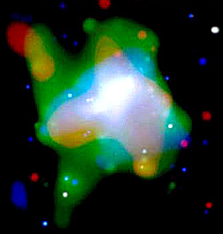
matter. There is growing evidence
that a significant fraction of the heavier elements were and are being produced
in the myriads of Dwarf Galaxies (most still undetected because of their reduced
luminosities) that pervade the Universe. Many of these undergo extended periods
of star formation and correlative supernovae bursts, releasing these elements
to intergalactic space. In this Chandra image of NGC 020724, a dwarf about 7
million light years away, giant bubbles of hot (10 million degrees) supernova
gases undergoing rapid expansion have been shown spectroscopically to contain
enrichments of oxygen, neon, magnesium and silicon.
Having now reviewed how
the elements are produced from Big Bang and subsequent stellar processes, we
should mention something about the relative abundances of the various elements
throughout the Universe. This turns out to be a difficult task for one obvious
reason. Spectroscopic measurements of elements from the distant stars are strongly
biased towards only those elements in excited states at or near the stellar
surface. Those elements principally in the interior do not contribute to surface
radiation in the same proportions as actually exist in a star. Only estimates
based on stellar interior models can be made. The situation is better for our
own star, the Sun. When element distributions are stated as Cosmic Abundances,
they actually are rough estimates made from Solar Abundances . And, the
latter abundances are not the same as the much better known Earth Abundances.
Below are two plots: Solar and Earth Abundances:
Note that the ordinate
for the Earth Abundance diagram is given in terms of mass fraction (all elements
together would make up 1, or 100%; note that Oxygen and Iron are the two most
abundant in/on/above the Earth). The Solar Abundance ordinate compares all elements
to Hydrogen (as scaled to an arbitrary H = 1012 atoms. We will take
a closer look at the left half of the Solar (Cosmic) Abundance curve with this
version
Several comments about
this (these) abundance plots are in order: First, the general trend is
towards ever decreasing abundances as the atomic number increases. Second,
there is a distinct zig-zag (up-down) pattern to the whole curve. For example,
between carbon and oxygen there is a decrease (the element is Nitrogen); between
neon and magnesium the decrease element is sodium; the largest drop is between
oxygen and neon, the element that thus decreases notably is fluorine. The reason
for this fluctuating pattern is just this: elements with odd numbers of nucleons
(protons and neutrons) are less stable, resulting in one unpaired (odd) proton
or neutron - those that pair these particles result in offsetting spins in opposite
directions that enhance stability (all this is part of the quantum theory of
nuclear arrangements). Third, there is a huge drop in abundance for the
Lithium-Beryllium-Boron (Li-Be-B) triplet. This results from two factors: 1)
At the Big Bang, nuclear processes that could fuse the proper H or He isotopes
into Li and/or the other two were statistically very rare and hence inefficient,
and 2) Some of the Li-Be-B that formed and survived may be destroyed in processes
with stars.
A somewhat easier task is
to compare stars and galaxies in terms of their metallicities - a ratio
of all amount of all elements with atomic numbers greater than 2 to the amount
of hydrogen present. Astronomers use the word "metal" differently from chemists.
A metal for a chemist includes only those elements in the Periodic Table labeled
IB through VIIIB. Astronomers simply include all elements (including those with
non-metallic properties) beyond He as "metals".
The "metal" composition
of the Sun is fairly well known. Actually, the measurements are made on the
chromosphere, the dominantly hydrogen gas which constitutes the solar atmosphere.
The source of spectral radiation, however, comes mainly from the photosphere.
The relative numbers of elements within the compressed body of the Sun is different,
but good estimates can be made based on element distribution models. One element
that gives many strong spectral lines is Iron (Fe). This element is chosen as
an indicator of the Sun's metallicity; it proxies for all metals whose amounts
tend to vary systematically with the iron concentration. Both the amount of
iron and of hydrogen present at the surface can be calculated from the strengths
of selected hydrogen and iron spectra derived from analysis of their absorption
lines as their quantized radiation passes through the chromosphere.
From these compositional data
a quantity determined as the ratio of amount of iron to amount of hydrogen (Fe/H)
can be calculated for the Sun. It is arbitrarily set = 1. Corresponding ratios
are determined for either individual stars or for galaxies (in which the Fe/H
depends on the gross or composite average of these two elements resulting from
radiation emitted by all stars, intragalactic gas, and halos within a given galaxy).
By convention, the Fe/H ratio values are expressed as log10 numbers.
This is a commonly used formula for comparing Fe/H ratios of stars to that of
the Sun:
Thus the Sun's Fe/H is
the log of 1 or 0. A star with a ratio of 1 to 100 yields a log value of -2;
this also means that the metals abundances are 1% of that established for the
Sun. A star whose log is +1 contains ten times as much metals as the Sun. Measurements
for thousands of stars have established that the range of log values is from
-4 (very metal-poor) to +1 (very metal-rich).
Some general observations
about the characteristics of stars as indicated by their metallicities: 1) the
disk portion of a galaxy has a range of metallicities, with Population I stars
having values > -1, i.e., towards smaller negative numbers to positive numbers
less than +1, whereas Population II stars have negative values beyond - 1; 2.
globular clusters and halo stars are metal-poor (values more negative than -1);
3) metal-rich stars are in the red segment of the Color Index and metal-poor stars
are blue; 4) although there can be complexities, in general metal-poor stars are
young in appearance (either near the outer limits of the Universe which show stars
that formed in the first few billion years after the Big Bang or stars formed
more recently from gas clouds that have had little contribution of heavier elements
from supernovae) and short-lived; 5) metal-rich stars from F, G, K, and M positions
on the Main Sequence are redder than stars of similar sizes (masses); and 6) dust
around a star will make it redder.
Overall, the rule of thumb
is just that a star will show a metallicity that depends on prior processes
that have changed the composition of the interstellar gas in the neighborhood
in which it forms. This is a function mainly of the number of supernovae that
have occurred previous to the formation of the star and the amounts of metals
each ejected that then became mixed into the cloud that supplies the star (and
other stars growing from this cloud). Since, over time the gas composition in
the interstellar medium should progressively enrich in metals, then those stars
that are metal-rich tend to have organized in later stages of a galaxy's history.
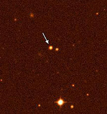
From the above it follows
that stars that are extremely metal-poor are likely to be first-generation and
thus primitive. HE0107-5240, a small star in our Milky Way some 36000 light
years from Earth, has an age estimated to be at least 12 billion years, making
it the oldest star examined to date. Here it is:
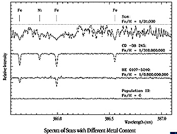
This star is extremely
metal-poor, as indicated by this series of spectra:
The ratio of Fe atoms to
H atoms for the Sun is 1/31000. The Fe/H ratio for HE0107-5240 is dramitically
lower, 1/6,800,000,000. Its composition then indicates that it had to form early
in Universe history when enrichment of the heavier elements had scarcely begun
in consequence of numerous early supernovae. Metallicity has a practical
significance to this Earth's inhabitants. Life does not apparently form around
all stars from O to M types. It tends to develop around those stars that will
produce planets of the right composition. Thus, the degree of element abundance
and enrichment become a vital factor. The dust around a star has a composition
that is related to the extent of metallicity found in that star. Only a small
fraction of all the stars is likely to have a suitable metallicity that extends
to its surrounding dust and gases, such that planets with Earthlike conditions
are produced. We were lucky. Now, putting the above
information on element production in the context of the existence of thinking
organisms: Life on Earth (and probably elsewhere) is based on carbon and a few
other elements (principally H, N, and O, but smaller amounts of P, S, and traces
of Fe and other heavier elements). Where does the carbon come from? As we have
already alluded to, scientists generally agree that matter was originally present
in the form of hydrogen, and that heavier elements up to Fe were constructed
by fusing together hydrogen nuclei (protons) with neutrons and electrons. This
process involves the conversion of a small amount of mass to energy, according
to Einstein's E = mc2. In the 1930s, Hans Bethe showed that the energy
radiated from the sun and stars could be produced by either or both of two sequences
of nuclear reactions: (1) the "proton cycle" in which protons are fused to form
helium nuclei (each having 2 protons and two neutrons); (2) the "carbon cycle"
in which a carbon nucleus (6 protons and 6 neutrons) absorbs a helium nucleus
to form an oxygen nucleus. But there did not seem to be any way to get from
helium to carbon. The most obvious path would be to combine two helium nuclei
to produce an isotope of beryllium with 4 protons and 4 neutrons, but that isotope
is not stable (it takes one more neutron to produce a stable isotope) and calculations
showed that it would not last long enough to pick up another helium nucleus
to yield carbon. However, in 1953 Fred Hoyle predicted that the carbon nucleus
has an excited state with just the right energy to match the energy of beryllium
plus helium, producing a resonance which allows the reaction to produce carbon
in the interior of a star. His prediction was confirmed by experiments at CalTech,
and the helium --> beryllium --> carbon reaction is now considered a crucial
step in a more general scheme of nuclear reactions that produce all the heavier
elements. Hoyle later noted that his prediction was a successful application
of the "anthropic principle": the Universe must have the properties needed to
allow the evolution of life, otherwise humans wouldn't be here to study it.
If some of the physical constants had slightly different values, the carbon
nucleus would not have an excited state with the right energy to make this reaction
go, and carbon-based life (especially us) could not exist. As a bottom line aside,
remember what we commented on in page 20-1: that the atoms and molecules making
up everything on Earth including our own bodies have had a continuous existence
from varying time spans in Universe history. Many elements have originated in
supernovae that fed material from our galaxy into the cloud leading to the organization
of the Sun and its planets. Hydrogen in the organisms of Earth, and in you particularly,
may trace the beginning of many (perhaps most) of the individual atoms in today's
life forms to the Big Bang itself. We truly are Star People. 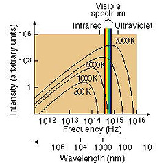
![]()
![]()
![]()