Without further ado, we now present
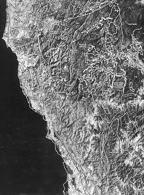
a two-image (September 1984), Landsat Thematic Mapper Band 3 mosaic that
includes the study area and mountains to its south, all the way to the
California border. We overlaid the terrane boundaries, redrawn from a regional
map, prepared by the U.S. Geological Survey, in white.
At first glance, and especially with
monitor limitations in mind, you may decide that differences in topographic expression
are hard to identify. But, to illustrate that these differences are really there
for some terranes, look at the two in the upper left, listed as Sixes River and
Elk. These terranes are clearly dissimilar, and, as we shall see in detail later,
they are the best case supporting the terrane-terrain hypothesis. Other terranes
with apparent differences relative to their neighbors include: Rogue Valley, Smith
River, and Yolla Bolly. Sixes River and Pickett Peak look too similar to identify
any distinctions.
The Smith River and Yolla Bolly terranes
also display differences in topography within themselves. Several areas within
the Smith River terrane near its upper left (northwest) border have apparently
high elevation and have more broadly spaced divides. These divides coincide
with a lithologic unit known as the Josephine ophiolite, which consists largely
of metamorphosed basalts or greenstones that represent parts of oceanic crust
that failed to subduct. Consider also three arbitrarily selected segments of
the Yolla Bolly terrane designated later in this survey as YbNorth (next to
the Snow Camp upper label), YbCentral (next to the Dry Butte label), and YbSouth
(next to the upper Smith River label). You should easily see differences in
the terrains (e.g., look for ridge or valley spacings). We will quantify these
differences later.
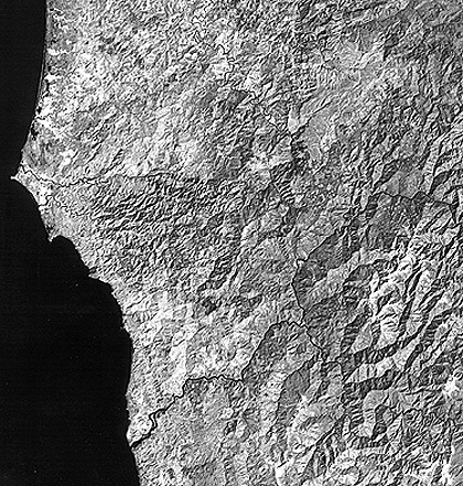
Let's take a closer look at the northwest
section of the mosaic, in this enlarged image. Let your eyes adjust to this image
and then try to draw imaginary boundaries around parts of it that seem separable.
Once more, the Sixes River-Elk pair of terranes leap out as different.
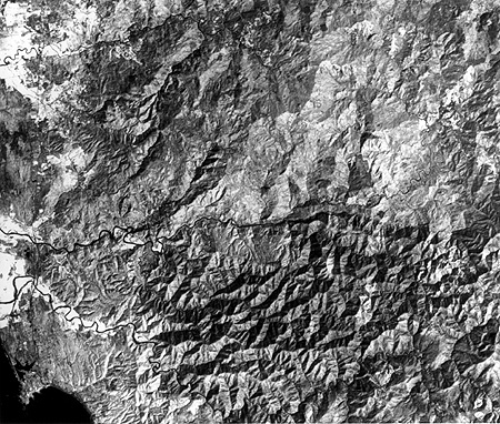
Now, we will enlarge the image even
further to focus on just the Sixes River and Elk terranes.
The upper and lower halves on the
right and center of this enlargement are conspicuously different. They are indeed
separable visually on the basis of topography. 17-18: What seems to be the most obvious
difference in this visual depiction of the two terranes? ANSWER
Geomorphic Parameters from Maps
What is responsible for the obvious differences? First, when we use DEM elevations
(in feet) for both terranes to compute the maximum height value in each square
mile and then fit a surface to these maxima, this plot results:
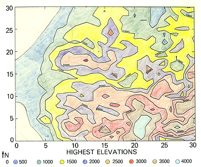
The boundary between the Sixes River (north) and Elk terranes runs horizontally across this map at approximately the middle. Clearly, the Elk terrane is on average at a notably higher elevation than the Sixes River terrane.
17-19: Which terrane is higher? ANSWER
Then, using a map (not shown) that plots the mountain ridges between valleys, initially drawn from contours on individual 15 ft topographic quadrangles and then merged into a single regional map, I calculated the total length of ridges per unit area (each a square mile). This is an indirect measure of ridge density. The average of two subunits in the Elk terrane is 5.16 (miles/square mile), whereas that for the Sixes River is 3.29. This suggests that the ridges are more closely spaced in the Elk terrane than in the Sixes River terrane, a conclusion borne out by simply looking at the enlarged Landsat images.
A third difference is not readily apparent from the images. But when the regional map of ridges are analyzed in terms of average direction of trend or orientation of ridges in square mile sampling units (a special computer program did this), resulting rose diagrams for each terrane indicate strikingly dissimilar patterns:
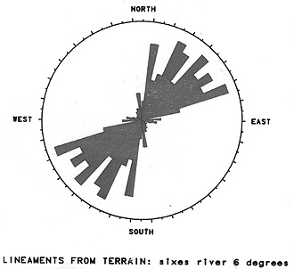
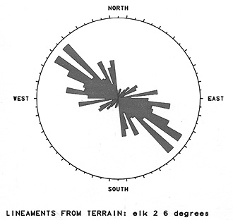
Most ridges in the Elk terrane trend northwest in contrast to the northeast trend dominating the Sixes River terrane. I'll give reasons for this later (for now, accept the idea that both ridges and stream valleys reflect structural control).
These ridge measurements, when made from topographic maps, are relatively unbiased, i.e., with careful work, we should record all the ridges that are bisectors of crest-proximate contours. This eliminates the inherent problem in space imagery and aerial photography of missing some linear features because of sun directional bias. Re-examining the Landsat imagery that we already saw indicates that the shadowing in this high-relief terrain, due to the morning Sun direction from the southeast, does emphasize the northeast trend of those ridges. But, when one looks at enlarged Landsat imagery, many of the ridges in other orientations can be detected by using tonal patterns related to moderated illumination differences along slope pairs that are not optimally oriented for easy discrimination. Still, inevitably some will be missed.
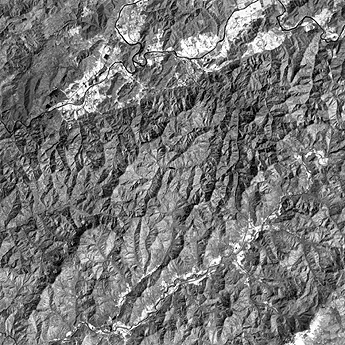
Stereo imagery pairs should reduce this bias effect. Two SPOT images made with the tiltable HRV scanner (see page 3-2), pointed at different angles and look directions on different dates, allowed us to map ridges directly from the imagery. Here is one of the (15 m [49 ft] resolution) panchromatic images (60 km [37 mi] on a side), covering the Gold Beach, Pickett Peak, and segments of the Sixes River and Yolla Bolly terranes:
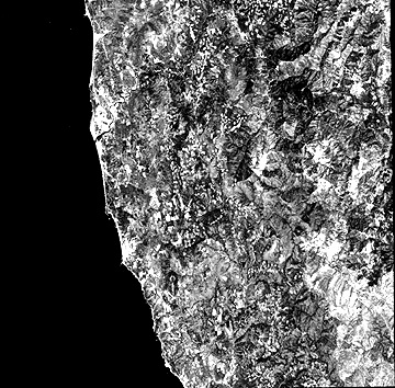
Although the higher resolution leads to more detail, the image appears flat, with the lack of strong shadowing inhibiting the expression of much of the topography. When viewed stereographically, the ridges associated with mountains of various heights do stand out well enough to foster tracing them onto a map.
17-20: The SPOT image contains a large number of light-toned, squarish "spots" (no pun intended). Any idea of what they might be? (Hint: think "forests"). ANSWER
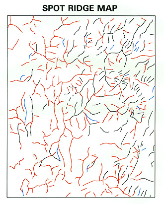
This next map shows all the ridges
mapped in SPOT and Landsat images in red. Green denotes extensions of ridges
selected from Landsat alone, and blue records images found only in SPOT. Surprisingly,
the use of SPOT does not seem to improve ridge detection by much. Perhaps the
Klamath terrain is well suited to depicting ridges effectively, even under the
morning sun conditions.
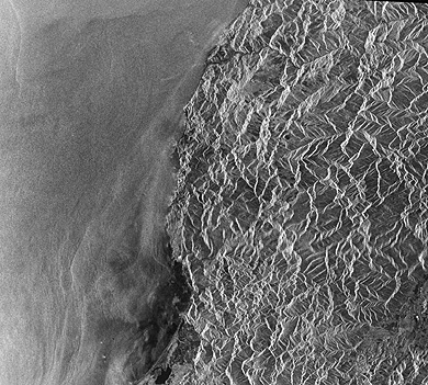
The same cannot be said for Seasat
radar imagery. This digitally correlated Synthetic Aperture Radar image, taken
in August of 1978, over part of the same areas as the SPOT image, indicates
the sensor is looking east, and as such, there is a pronounced slant-range distortion
that results in foreshortening layover. The image introduces a notable bias,
that highlights the bulk of ridges oriented north-north-east and misses many
others completely. A data product in this form is not suited to orientation
analysis.
Look now at two terranes - Rogue Valley and Yolla Bolly - that appear similar at their northern end, as evident in this enlargement (with a locator sketch map) (we don’t comment on the Sixes River and Snow Camp terranes north of the Canyonville fault):
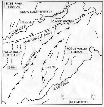
A right lateral strike-slip fault bounds both terranes (i.e., the northern block moves right, relative to slippage to the left in the lower block) near Canyonville. The terranes are juxtaposed along a large thrust fault, inclined downward to the east, resulting where the Yolla Bolly terrane slid under the Rogue Valley. At a quick glance, the ridge spacing and relief for the mountains in each terrane near this fault seem similar. The ridge orientations of the Rogue Valley terrane are more northward than those of Yolla Bolly.
17-21: In visually examining these two terranes in the above Landsat subscene, do you notice any difference(s) besides ridge orientation? ANSWER
One difference is not evident from
visual inspection but comes out when one makes measurements from the Canyonville
topographic sheet. Arbitrarily, I read the highest elevation in each township
section (1 square mile) from that map. When plotted as a histogram (frequency
of maximum elevations), the following distribution results:
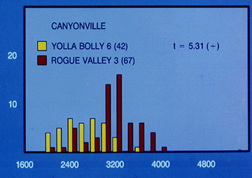
Allowing for the difference in the number of data points involved (67 versus 42), there still is a notable variance between height distributions. In this topo sheet, the average maximum elevation in the Rogue Valley terrane is 984 m (3,226 feet), whereas in the Yolla Bolly terrane, it is 845 m (2,774 ft). Treating these two sets of measurements as two distinct populations, a statistical device known as Student's t-test gave a value of 5.31, which is significant (i.e., shows a real difference) at the 99% confidence level. I surmised that this dual distinction results from differences in dominant lithologies. The Yolla Bolly is characterized by siliceous shales, and the Rogue Valley includes more resistant rock types.