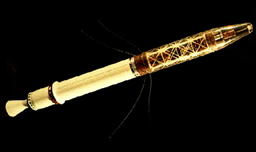
Instead of the more conventional-looking
satellites (most with thrusters to adjust their orbits) that we shall depict
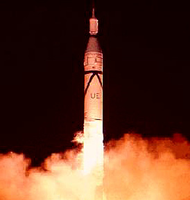
throughout this Tutorial, Explorer 1 itself was a small rocket with its own
engine. It was thus actually the fourth stage of the rocket assembly. Here is
a picture (against a black background to simulate the darkness of space).
This 4th stage was 2.03 m (6.67
ft) long and 15 cm (6 inches) wide. Its bottom contained fuel for getting the
entire assembly into orbit. The payload - scientific instruments including a
cosmic ray detector, micrometeorite package, and several temperature sensors
- was mounted in the cross-lattice frame. The top was protected by a nose cone
shroud. Once in orbit, this assembly rotated rapidly. Explorer 1 functioned
successfully for 3 months until its batteries gave out.
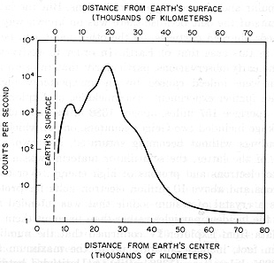
Explorer 1 made a major discovery
about the interaction between the Earth's geomagnetic field and incoming charged
particles from the Sun and outer space. A team headed by Dr. James Van Allen put
together an instrument package centered on a Geiger counter suited to measuring
variations in particle radiation. As it orbited, Explorer 1 repeatedly passed
through a region in which the amount of radiation increased significantly. When
Pioneer 3 was placed in a highly elliptical orbit in December 1958, it was determined
that there were actually two peaks in counts as shown in this plot.
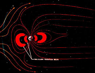
These zones of increased intensity
proved to be due to trapped particles held in the Earth's magnetic field. They
were concentrated in two torus or doughnut-shaped zones that were named the
Inner and Outer Van Allen Belts. This illustration is a two-dimensional cutaway
sketch of streamlines representing solar wind particles as they passed through
Earth's magnetic field.
The Inner V.A. Belt reaches its
maximum intensity at 5000 km (3000 miles) but extends inward to about 1000 km
(600 miles) The Outer Belt starts at 1500 km (9300 miles) and peaks at 22000
km (15500 miles). That belt is dominated by trapped electrons from the solar
wind; the Inner Belt is marked by protons brought in mainly as cosmic rays.
Two important conclusions from the discovery of the Van Allen Belts: 1) they
have for eons provided protection from these potentially devastating particle
bombardments - a fact critical to the successful development of life on Earth;
and 2) both spacecraft and humans would need to be shielded effectively when
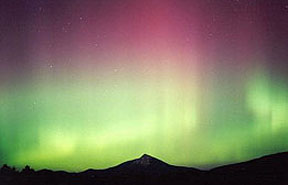
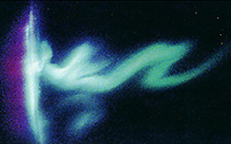
passing through the Belts. The Van Allen Belts become much
weaker above 75°N and 75°S. This allows more particles to reach the the upper
atmosphere and collide with oxygen, nitrogen and argon atoms in the air to generate
ions that in their excited states give off constantly moving, colorful, wavy
displays known as the aurora borealis in the northern hemisphere and
the aurora australis in the southern hemisphere. This geophysical phenomenon
occurs mainly at the higher latitudes but sometimes extends below 40°; it is
seen most frequently around 70° latitudes. The first image below shows the aurora
as photographed on the ground in Colorado and the second image was taken by
astronauts from the Space Shuttle.
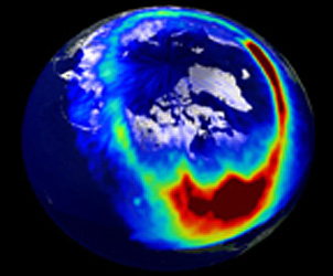
An example of symbiosis in remote
sensing is this: A satellite named SOHO whose job is to monitor solar activity
reported intense solar storms in mid-July. This was predicted to produce a spectacular
aurora borealis flare-up visible as far south as the northern U.S. Unfavorable
viewing conditions caused rather subdued displays. But, a NASA satellite called
Polar (launched in 1996) designed to monitor just such phenomena produced this
view in the visible from space:
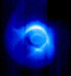
In recent years, some spectacular
images of the particle-trapping fields around the entire Earth have been taken
by sensors on satellites placed in highly elliptical orbits or at Lagrangian
points (where Earth-Sun gravitational forces balance out) or enroute to the
Sun or other distant bodies. In the top image, the Earth's radiation field in
the excited atmosphere is seen in the Extreme Ultraviolet (EUV) part of the
spectrum by the IMAGE (Imager for Magnetopause to Aurora Global Exploration)
satellite; the shape of this field is determined largely by the Earth's magnetic
field (note the trailing pattern, related to the geomagnetic tail [see below].
The arc-shaped inner belt is now called the plasmasphere. The distribution of
the trapped solar particles in this image is strongly controlled by the Earth's
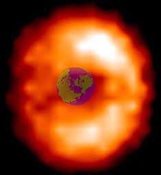
magnetosphere (see below). The lower image is made by the HENA (High Energy
Neutral Atom) sensor to show density variations of a hot plasma surrounding
Earth.
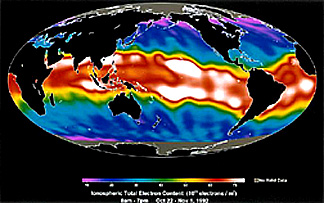
Many satellites have been placed in
space by various nations to get global scale data on the Earth's magnetosphere
and its the ionosphere (a globe-circling band located largely between 80-400 km
[50-250 miles] above the surface, containing electrons stripped by gamma rays
from nitrogen and oxygen). Here is a plot of the global distribution of the ionosphere,
measured by the Jason-1 satellite (pages 8-7 and 14-12) whose prime mission is
to measure Sea Surface Heights.
Other satellites have made countless
measurements and observations of the inner atmosphere (about 97% by mass of its
gases [about 78% N2, 21% O2, 0.93% A(rgon), 0.35% CO2]).
The atmosphere tends to be homogeneous (mixed uniformly) within the bottom (near
surface) 30 km (18 miles). The upper thin atmosphere extends out to about 120
km (75 miles). At greater distances outward the gases separate into shells (the
heterosphere) with the innermost being molecular nitrogen, then atomic oxygen,
then atomic helium, and a thick (from 3500-10000 km [2200-6000 miles]) outermost
layer of atomic hydrogen. (See Section 14 for a fuller treatment of meteorological
remote sensing of the lower atmosphere.)
Much was learned about the Earth's
natural environment above its surface - both in regards to the nature and distribution
of particles and fields and to the various atmospheric zones - in the first
decade of the space program. Of special note is the OGO (Orbiting Geophysical
Observatory) series, of which 6 were launched in the 1960s. Three of these have
nearly polar orbits and are sometimes referred to as POGOs. Satellites have been the main tool
for measuring the terrestrial geopotential fields at global scales. This includes
such physical properties as regional magnetic and gravity variations or anomalies
originating within the solid Earth but expressed at the surface. In particular,
such properties are more difficult to measure under the oceans but data derived
from satellites provide the means to determine the distribution of magnetic
and gravity differences over large tracts. The magnetic field varies over time
but the gravity field is almost completely time invariant.
The Earth's dipolar geomagnetic
field (first examined scientifically by W. Gilbert in 1600) results from slow
motions in its fluid Outer Core (the Inner Core is very hot, under extreme pressure,
but solid). The movement is powered by the Earth's rotation and by thermal gradients.
Detached electrons from the Iron-Nickel core material produce electric currents
that through the dynamo effect generate the magnetic field (which can be depicted
by lines of force) that presently emanates from the Earth's South to its North
magnetic poles. (This phenomenon of magnetic field generation was discovered by
H.C. Oersted in 1819 quite serendipitously during a demonstration of electric
currents to his students; the needle of a compass lying nearby moved when the
current flowed, from which he deduced this cause-effect relation.)
The geomagnetic field (derivative
from the lines of force data) is composed of three parts: 1) the Main Field,
caused by the internal processes in the core, which accounts for more than 95%
of the total field strength; 2) the External Field, resulting from processes
in the ionosphere leading to a superimposed field; and 3) the Anomalous Induced
Field, caused by induced (secondary) magnetism generated in iron minerals (such
as magnetite and hematite) found mainly in the crust, including those substances
that have an inherited remanent (permanently induced) magnetism; these give
rise to local variations called anomalies that tell geophysicists and
prospectors about localized to regional concentrations of certain rock types
and possible commercial minerals. The geomagnetic field strength is commonly
plotted in intensity units. The basic unit is the oersted (1 dyne per
unit pole), which is numerically equivalent to the gauss, the preferred
term when magnetic induction is measured. A derivative unit is the γ, which
is 10-5 gauss. In the SI units system, intensity is measured in Teslas
(defined in units of Newtons/Ampere-meter) or more commonly nanoTeslas (nT;
10-9 Teslas); an nT is the equivalent of the γ. Although more complicated in its
details, the Earth's geomagnetic field can be likened to that associated with
a simple, straight bar magnet, as pictured thusly:
This pattern of symmetrical lines
of force (the magnetic flux) is idealized to describe the concept. Actually,
the main geomagnetic field is much distorted by interaction with the solar wind
(a plasma of particles from the Sun driven outward at high speeds) which exerts
a "pressure" on the field compressing it on the side facing the Sun and drawing
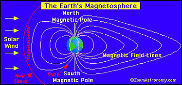
it out in a streamlined elongation away from the Sun. In two dimensions, the
modified field appears like this, as determined from satellite measurements:
The region around Earth in which
the terrestrial magnetic field is enclosed by the solar wind is termed the geomagnetic
cavity. The outer cavity is bound by the magnetopause. Where the
solar wind encounters the magnetosphere on the Sun-facing side, a magnetohydrodynamic
bow shock wave is produced as much of the solar wind is deflected around
the magnetopause. On that side, the region between the bow shock front and the
magnetopause is called the magnetosheath. Behind the Earth, on its nightside,
the magnetic lines of force are stretched out into the magnetic tail
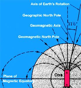
which extends for well over 150,000 km. Note that the magnetic and the rotational
poles are currently about 11° apart. Both poles wander (precess) so that this
angle changes with time. The angle between true North and magnetic north, or
between the geographic and magnetic meridians, is called the magnetic declination.
The angle between the path of a magnetic line of force at some latitude and
the horizontal is the magnetic inclination (it can be determined locally
with a magnetic dip needle [held vertically]). The angle is zero at the magnetic
equator (field line parallel to the surface, 90° at the poles, and at intermediate
angles between these two reference positions. Both declination and inclination
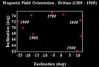
shift globally or in a region over time; long-period variations in direction
and intensity are called secular changes. This effect is shown here for
nearly four centuries of ground-based data from Great Britain:
Variations in magnetic inclination,
declination, total intensity, and horizontal and vertical intensity vectors
can be determined from ground and space measurements. Over the years, these
have become part of the geomagnetic community's data base called the International
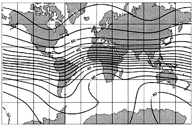
Geomagnetic Reference Field (IGRF), now updated every four years. Here is a
global plot of the general geospatial distribution of magnetic inclination values
for 1995.
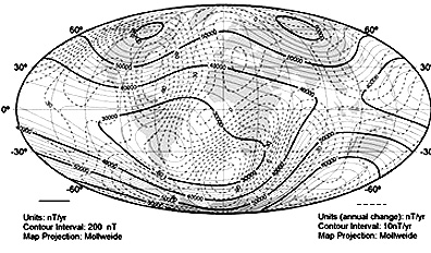
The total magnetic field as determined
by satellite measurements can be shown in this global diagram, with the solid
black lines representing intensity values and the dashed lines denoting typical
annual variations, both plotted in units of nanoTeslas (nT).
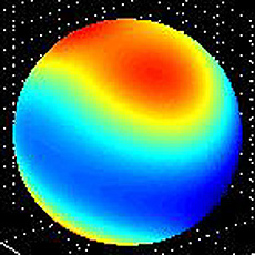
The geomagnetic measurements have
confirmed and refined our knowledge of the magnitudes and distribution of global
intensities. These range from about 25000 nT at the equator to 65000 nT at the
poles (or from 0.25 to 0.65 gauss). This next illustration is a general depiction
of this variation (low values in blue; high in red):
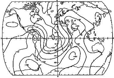
The secular variation in intensity
can be as much as 150 nT per year. Here is a global map of cumulate changes
during the years 1925-27 as determined from many ground stations:
Geomagnetic measurements were among
the first geophysical data acquired by early American satellites such as several
Explorers, Pioneer I and V, IMP-I, and the OGO series and by such Russian satellites
as the first two in the Lunik series that also went to the Moon. A major advance
in surveying geomagnetic anomalies was made by Magsat, launched in 1979.
Although data collection was short-lived owing to the limited duration of the
mission which ended in June 1980, the spacecraft operated long enough to provide
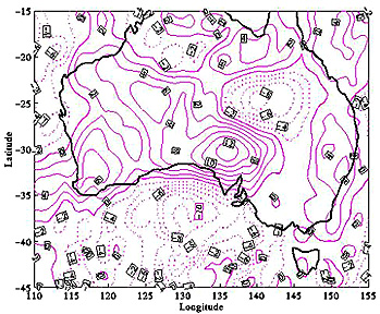
an invaluable set of measurements still being examined 20 years later. Here,
for example, is a 1995-produced map of variations in intensity over most of
Australia.
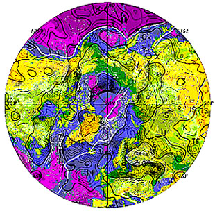
When produced as color-coded maps,
Magsat-determined intensity variations are impressive in their detail. This
map was made to cover the North polar region:
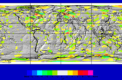
Major anomalies worldwide were identified
by Magsat. This map shows significant anomalies (in nT, ranging from -12 in blue
to +12 in pink) plotted on a topographic/bathymetric base as a gray background
with some first order surface features superimposed. One of particular interest
is the Central African Anomaly (blue area low just above the red area high).
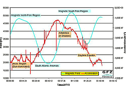
Since the Magsat benchmark mission,
other satellites have, or will be, orbited to monitor and improve the geomagnetic
properties measured conveniently from space. These include POGS (Polar Orbiting
Geomagnetic Survey) in 1990, Oersted (a Danish mission; 1999), Champ (German;
2000), and SAC-C (Argentina; 2000). Champ, as an example, makes both magnetic
and gravity (acceleration) measurements:
We would be remiss if the
essential results of years of paleomagnetic studies were not included
here. While satellite data support this work, they are not the prime means by
which knowledge of the history of changes in the Earth's magnetic field is obtained.
This has been done mainly through ground sampling of rocks collected on the
continents or from the oceans' floor. This approach is not remote sensing in
strictu senso but it does lead to reconstruction of magnetic field geometry
at global scales that assumed different orientations in the past. And, it provides
an "excuse" to introduce into this Tutorial a review of the now fully accepted
paradigm called Plate Tectonics which dominates models of the Earth's
geologic history and modes of operation. That will serve as background for remote
sensing topics covered in several Sections dealing largely with geologic applications.
The basis underlying paleomagnetism
is the discovery that the magnetic field shifts its polarity with a rather irregular
periodicity over tens to hundreds of thousands of years. Thus today's North geomagnetic
pole (in which the magnetic lines of force enter Earth from space) has been a
South pole (from which the lines emerge) many times in the past. This switching
back and forth of the N and S magnetic poles relative to Earth's North rotational
pole is termed magnetic reversal. When the two North's coincide, the present-day
polarity is arbitrarily said to be normal; when the South magnetic pole
is located near the North rotational pole, polarity is reverse. It is possible
to determine polarity at a given time in the past (as determined by radiometric
dating) by measuring the polarity of a rock sample containing ferromagnetic mineral(s).
Magnetite, Fe3O4, is most frequently used. Magnetite is
one of the first accessory minerals to crystallize in a basaltic magma/lava. As
the magma temperature drops through 580° C, magnetite passes through the Curie
point, at which it takes on its magnetic orientation, becoming like a dipolar
"needle". During continued cooling, magnetite grains will orient their N-S polar
axis, much like a compass, such that the north pole of a crystal will align with
the lines of force and will point to where the geomagnetic North pole was at the
time when the crystal was "frozen" in place as the magma solidified. The process
by which this occurs is called thermoremanent magnetism.
The application is this:
Continental basalts (and sometimes sedimentary rocks) containing magnetite are
sampled in the field, usually by coring, with the core's spatial position established
by fixing its three-dimensional orientation. The (radiometrically dated) sample
is then examined for magnetic orientation in the laboratory (referenced to its
field position). This determines the alignment (direction and inclination) of
the permanent magnetic field imposed on the magnetite before rock consolidation
at the time well into the past when the lava was extruded or sediment deposited.
This paleomagnetic field geometry points to some position on the Earth (relative
to today's geography) that represented an apparent location of the poles
at the time of the rock's age. Furthermore, the polarity (normal or reversed)
could also be determined. The same technique, and resulting information, could
be applied to oriented basaltic rocks beneath ocean floor sediments that were
retrieved by core drilling. Two major discoveries, vital to developing the concepts
of plate tectonics and continental drift, gradually emerged through the 1960s
to the present. The first is sea floor
spreading. Through deeper parts of the several ocean basins, volcanic upwelling
has build long, relatively narrow rises or ridges which today are sites of active
marine volcanism. Lavas emerging today take on the normal polarity that has
persisted over the last 700,000 years. When recovered as cores, the solid basalts
have magnetic orientations consistent with modern pole locations. But, as sampling
moves away laterally from the ridges, the basalts become progressively older.
When their polarities are determined, a pattern of alternating polarities (normal-reverse-normal-reverse-normal.....)
emerges. Actually, this state was initially determined by geomagnetic surveys
using magnetometers towed behind ships. Even more remarkably, the pattern on
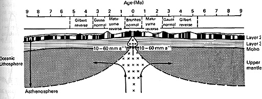
one side of the ridge is matched by a pattern on the opposite side. This diagram
should clarify the observation (black is normal polarity; white is reverse):
The figure
shows normal-reverse patterns for the last 9 million years (horizontal top scale).
The current and the three most recent magnetic epochs are named. Average rates
of plate movement are shown by arrows. The N-R patterns are repeated in samples
from all the oceans, so that the polarity shifts are clearly global in effect.
These distinctive patterns form the basis of a geomagnetic age dating method
that has been proven to work well. There is enough variation and uniqueness
in the patterns to allow suites of rocks formed over a span of several million
years or so to be placed at a certain age if they include several reversals.
This magnetochronology has been carried back into the Cretaceous Period some
100+ million years ago.
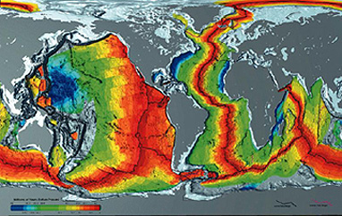
Enough radiometric ages
collected at many locations within the sea floors of the different named oceans
have been determined to allow maps of relative age to be produced for the entire
globe. Here is one in which the youngest ages are in red and oldest in blue
(thus the blue regions were formed first and have been driven away from the
ridges towards plate boundaries). It follows that the seafloor is everywhere
relatively young inasmuch as older basaltic units at sea floors of pre-Cretaceous
age have been destroyed by subduction (see below):
As the ages of
basalt lavas were determined, and it became evident that the extruded lavas
became progressively older moving towards continental land masses on either
side of the ridge, a mechanism to explain these patterns was proposed independently
by H. Hess and R. Dietz. Sea floor spreading postulates that lavas from the
oceanic crust or mantle rise to the surface at the ridge, pour out, and push
laterally against two lithospheric plates (oceanic crust plus the top of the
Upper Mantle) on either side. This is more or less continuous for long times.
The plates slide along the asthenosphere (region of the Upper Mantle hot enough
for the rocks to act as though viscous, almost liquid material) in a motion
likened to a conveyor belt until they encounter a boundary with another plate.
(There are 7 major plates and a larger number of smaller plates; see of this
Introduction or the top of page 17-3 for a global
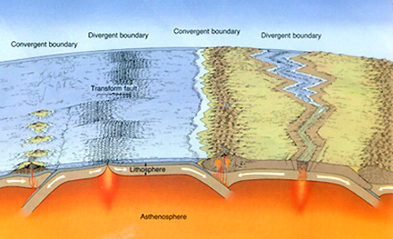
map of these plates). Several different responses are possible at these boundaries,
as shown in this next diagram which summarizes much of the main idea behind
plate tectonics.
A Mid-Ocean ridge appears at the
left divergent boundary, from which lithospheric plates move in opposite directions.
The ridge is cut by a number of transform faults which break the plate into
segments. A series of slight rises are evident. Each may be associated with
a magnetic reversal. At the far left is one type of convergent boundary - where
two oceanic plates approach each other. One plate is driven downward (subduction)
beneath the other into the mantle, gradually melting as it gets deeper. Some
of the molten rock reaches the surface to form a chain of volcanic islands (and
sediment) called an Island Arc (Indonesia is an example). The right moving plate
moves against a convergent boundary located at/near the edge of an embedded
continental assemblage of rocks on its own plate. Above its subduction zone,
melted rock and tectonic upwelling and compression produce folded sedimentary
rocks and volcanic and plutonic (magmas that intrude rocks above but don't reach
the surface) rocks to form one or more mountain chains (the Coast Ranges and
Sierra Nevada/Cascades along the western part of the U.S. are an example). In
this idealized diagram, the continent-bearing plate is shown as splitting along
a rift zone formed along another type of divergent boundary. The plate to its
right is moving against another plate that has a second continent in its crustal
portion; again mountains are developed by folding, faulting, and intrusion (the
Himalayas against the Indian subcontinent are an example). One might wonder now about the mass
balance associated with the plate movements. As a plate is heated up during
subduction, it (at least partially) melts. Some of that now fluidized material
is moved laterally back towards one or more spreading ridges. Thus, a closed
cycle of moving rock and magma results. The process is aided by 1-2 sets of
circulating convection currents in the Mantle which provide the energy to power
the cycle. Possibly some convection occurs above the crust-mantle boundary (the
so-called Mojo) and may couple with the drag applied by the upper convective
movements that affect a lithospheric plate from below. Now to the second discovery: Polar
Wandering. When oriented rock samples are analyzed to determine where their
magnetic components are pointing to where the magnetic pole was located at the
time of their formation, rocks of different ages are found to have polar locations
in different parts of the present-day world. One might surmise that the magnetic
poles have wandered over much of the globe relative to its rotational poles.
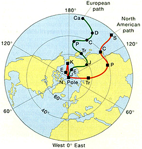
This next figure shows plots of magnetic pole positions on a modern geographic
grid (latitude-longitude) for the northern hemisphere, with the age of the rocks
involved shown by letters (from oldest to youngest: Ca = Cambrian; S = Silurian;
D = Devonian; C = Carboniferous; P = Permian; T = Triassic; J = Jurassic; K
= Cretaceous; E = Eocene); For a table showing the geologic time scale, with
assigned ages, click here).
The poles occupied different positions
from the Paleozoic onward until the Present (and still other positions in the
Precambrian). One might surmise that the poles were indeed in different locations
on the Earth's surface at various times in the past, but that would be hard to
explain since the magnetic poles apparently have always been close to the rotational
poles owing to the mechanism of magnetic field generation that assumes the electrical
currents in the Outer Core move generally subparallel to the Equator. And, it
seems odd to have two sets of pole patterns in North America and Europe, moving
approximately along similar paths, but separated (offset) from each other.
The answer to this duality conundrum
is tied to the concept of continental drift . At various times in the past,
the continents did not have their present shapes (beyond their sealevel outlines)
or relative positions. In fact, continental crustal masses have been joined into
one or more supercontinents (since the Late Paleozoic Pangaea, which split into
Gondwana and Laurasia that then divided further into the present-day continents)
several times. As a supercontinent comes apart, its new pieces move across the
globe embedded in wandering crustal plates. Pangaea itself resulted from collisions
of plates bearing earlier continental masses which were welded together, only
to then resplit later; evidence suggests there were similar large supercontinents
of different shapes/sizes and locations during Early Paleozoic and Precambrian
times.
If the North American and European
continents were relocated over time back to their Early Paleozoic positions, the
two curves in the above figure will almost superimpose. This is strong proof of
the drift hypothesis.
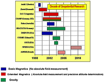
As a transition to a topic -gravity
- covered in the next page, we show now a summary of recently orbited and planned
magnetic and gravity measuring satellites for the first decade of the 21st Century: