| back |

|
next |
PAPER-1
A GIS BASED INTEGRATED MODEL FOR ASSESSMENT OF HYDROLOGICAL CHANGES DUE TO LAND USE MODIFICATIONS
S. Mohan and Madhav Narayan Shrestha
| back |
|
next |
| ABSTRACT: | up | previous | next | last |
In this paper, a distributed hydrological model with SCS (Soil Conservation Service) curve number method (CN) is developed to assess the hydrological changes due to land use modification in a basin. The method is developed for assessment of CN in micro level of land use, which is an efficient tool to evaluate the land use modification. Kathmandu Valley basin, Nepal, has been chosen as a case study. The forecast of the runoff can be made by Land use change (LuC) model for known change in land use and is useful to quantify the effect due to this change. The sensitivity analysis performed in this study shows that for agriculture dominated hilly watershed, the value of initial abstraction ratios are found to be 0.27, 0.2 and 0.17 for pre monsoon, monsoon and post monsoon seasons respectively. For the study area, it was found that the peak runoff value increased by 12.7 %, 6.5 % and 5.3 % during monsoon, post-monsoon and pre-monsoon respectively for 9% deforestation and 17 % urbanization. The study clearly demonstrated that integration of remote sensing, GIS, HEC-1 and spatially distributed hydrological model provides a powerful tool for assessment of the hydrological effect due to land use modifications.
| INTRODUCTION: | up | previous | next | last |
There has been a growing need to quantify the impacts of land use changes on hydrology from the standpoint of anticipating and minimising potential environmental impacts. Watersheds may be modeled by a lumped model using basin average input data and producing total basin stream flow. Such a model may produce reasonable result, but because of the distributed nature of hydrological properties like soil type, slope and land use, the model cannot be expected to accurately represent the watershed conditions. The conventional methods of detecting land use changes are costly and low in accuracy. Remote sensing technique, because of its capability of synoptic viewing and repetitive coverage, provides useful information on land use dynamics. With the development of GIS and remote sensing techniques, the hydrological catchment models have been more physically based and distributed to enumerate various interactive hydrological processes considering spatial heterogeneity. The purpose of this study is to develop a spatially distributed hydrological model, which can be used to assess the effects of land use change. The model is developed based on Soil Conservation Service-Curve Number (SCS- CN) approach.
| EARLIER WORKS: | up | previous | next | last |
The changes in land use due to natural and human activities can be observed using current and archived remotely sensed data. Although originally SCS-CN method was developed for agricultural purpose, the method has been expanded for use in urban and suburban areas. The method is attractive, as the major input parameters are defined in terms of land use and soil type. The advantage of the method is that the user can experiment with changes in land use and assess their impact. The procedure is most satisfactory, when used for hydrologic problems that are designed for the evaluation of land use changes.
Many investigators predicted runoff using SCS-CN method, which resulted in the best prediction of yearly runoff volumes. The GIS and SCS-CN methods were combined with the model rainfall-runoff relations and the watershed parameters were estimated using ARC/INFO while computation of other parameters required significant user interaction. (Stuebe and Douglas, 1991; White Dale, 1988; Hill, et al., 1987; Bhaskar, et al, 1992). The application of SCS-CN method is widely used for different studies such as reclamation of surface coal mines (Ritter, et al., 1991), urban storm water modeling (Tsihrintzis and Hamid, 1997; Greene and Cruise, 1995; Meyer, et al., 1993), impoundment watershed modeling (Schoof, 1983), etc. They found that the method was suitable and able to quickly respond to estimate runoff with lumped parameters.
The lumped parameter hydrologic models were developed with GIS for computing rainfall-runoff process from different land use classes (Kite and Kauwen, 1992; Hellweger and Maidment, 1999). They did not consider data describing soil parameters and found that using a semi-distributed model resulted in better goodness of fit than the lumped basin approach. The semi-distributed hydrological models were also developed using GIS for a limited consideration of spatial heterogeneity and successfully applied for estimation of model parameters (Schumann, 1993; Suwanwerakamtorn, 1994; Purwanto and Donker, 1991). The model was used to assess the effect of land use change for hypothetical cases of reforestation and deforestation conditions. When hypothetical case of 5% reforestation or deforestation conditions were considered, the peak flow reduced by 14 % for reforestation and increased by 12 % for deforestation case for hydrologic soil group C when compared to normal land use.
The focus of the research by the aforementioned investigators was mostly in developing or extracting attribute data for geographic features or hydrologic elements to support lumped or semi-distributed hydrologic modeling. The estimation of parameters for the model was carried out mostly considering fixed representative size of land use at either grid-cell level or sub-catchment level. Spatial heterogeneity of the land use at micro level has not yet been considered in hydrologic modeling. In this paper, the focus is on spatially distributed modeling considering three-dimensional physiographic heterogeneity in terms of topography, soil, and land use. The model will assess the hydrological change due to land use modification, which is a most essential study for 21st century with the problem of rapidly growing urbanization, or land use modifications. The model will serve as an efficient tool for land use management.
| METHODOLOGY: | up | previous | next | last |
The method for evaluating the hydrological change due to land use modifications can be implemented by integrating remote sensing, GIS and HEC-1 Model (The Hydrologic Engineering Center, 1981). A system approach is essential to analyse and model the hydrological dynamics of heterogeneously structured drainage basin. Three-dimensional physiographic heterogeneity in terms of topography, soil and land use can be grouped together into associations. These associations are defined here as Hydrological Similar Units (Ott, et al., 1991). Hydrological Similar Units (HSU) are homogeneous structured areas with same land use and pedo-topo-geological conditions controlling their unique hydrological dynamics. The derived applicable characteristics from different sources are used to derive the HSU and the hydrological changes due to land use modifications are assessed as described in Fig.1. From satellite image data (LandsatTM and ADEOS), the visual image interpretation is carried out using an interpretation key generated through field survey. The ground checks were made for confirming the land use units. Whereas, the spatial database containing information on land use, soils type, topography, hydraulic characteristics and meteorological information is created using PC-ARC/INFO from topographical map.
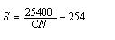
Appropriate curve numbers (CNs) according to standard tables (Soil Conservation Service, 1972) are assigned to each HSUs considering antecedent moisture conditions (AMC). Then the direct runoff values from each HSUs are estimated using SCS-CN method for rainfall events. The cumulative runoff from the basin outlet is calculated using HEC-1 model and compared with observed runoff for that period. Effect of land use changes is evaluated for different periods by quantifying the runoff and the lag time. In developing the relationship for Q (runoff depth), the Soil Conservation Service (1972) developed the expression as,
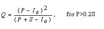
Q = 0, for P� 0.2S (1)
Where P = total rainfall and S = potential retention or infiltration. The Eq. 1 was derived for Ia, initial abstraction taken as lS, where l is an initial abstraction ratio. l has to be found out by sensitivity analysis. The variable S, which varies with antecedent soil moisture and other variables, can be estimated as;
 (2)
(2)
CN values are in a range from 0 to 100, with higher CNs associated with higher runoff potential watershed. To evaluate proper CN values, the soil of the basin is classified into four Hydrologic Soil Groups (HSG) based on their minimum infiltration rate (SCS national engineering handbook, 1985). The changes in land use will be evaluated by accounting the HSU distribution over the entire area for different periods, which in turn would give the changes in CN over the period considered. The changes in the runoff and runoff lag time are computed using Eqs. (1) and (2).
| STUDY AREA: | up | previous | next | last |
Kathmandu Valley in Nepal has been considered for the study (Fig.2). The valley is a roughly circular bowl shaped intramontane basin of 651 km2 lying between 27� 32' N to 27� 49' N and 85� 11' to 85� 32' E. Bagmati is the main river which originates from north and flows towards south-west and forms a typical centripetal drainage system. It passes through Chovar gorge, which is the only outlet of the basin as shown in Fig.3. The climate of the valley is subtropical to monsoon with hot and wet summer and cold and fairly dry winter. The maximum and minimum temperatures are 350C and -2.50C respectively. About 80% of the total annual rainfall occurs during the months of June to September. Winter rainfall is common but not heavy. The average annual rainfall in the basin is 1600 mm. The valley consists of three administrative districts namely, Kathmandu, Lalitpur and Bhaktapur. A part of the present study area lies in all the three districts.
| DATA AVAILABILITY AND DEVELOPMENT: | up | previous | next | last |
The base map as well as the land use map for the year 1978 is derived from topomaps using PC ARC/INFO. Digital images for 1984 (Landsat TM), 1990 (Landsat TM) and 1996 (ADEOS, AVNIR Japan) are used. Visual image interpretation of satellite data is carried out using an interpretation key generated through field survey and verifications. The daily and monthly rainfall record of 9 raingauge stations for period 1965 to 1996 are collected. The monthly and daily data available for the five stream gauging stations, namely Chovar, Gaurighat, Buddhanilkantha, Sundarijal and Tika Bhairab are collected. Some missing records of rainfall are filled in considering the correlation structure with other stations. The correlation coefficients are in between 0.873 and 0.966. The missing stream flow data are filled up using 'LAST' model (Lane and Frevert, 1990), which is a multisite generation software package which preserves serial and cross correlation with multi lag linear autoregressive model. The completed flow data for Sundarijal station is compared statistically up to fourth moments with available records. It is found that the generated flows maintain the historical statistics and are satisfactory with slight deviation on low flow periods.
| ANALYSIS OF RESULTS: | up | previous | next | last |
Land use, hydrologic soil group (HSG) and slope coverages are overlaid using GIS ARC/INFO. A complete GIS database is made. There are four types of HSG, 7 types of land use and five ranges of slope in the study area. Considering different combinations, twenty-five types of HSUs are derived. HSU type with different land use, slope and HSG are presented in Table 1. HSU type 11 and 15 are not found in the area. Total numbers of HSUs derived are 1119, 1291, 1375 and 1407 for 1978, 1984, 1990 and 1996 respectively. The minimum delineation of area observed is 8 m2.
In the study area, forest (mountainous) area is about 30 % of the total basin area and the remaining area (70%) has an average slope of 0 to 4%. Some subbasins have forest area of less than 3 %. Thus, the average orographic influence on the rainfall can be neglected for estimation of aerial rainfall. The available rainfall recording stations are insufficient to prepare isohyetal maps. Both rainfall depth and spatial distribution for each sub-basin are taken by Thiessen Polygon method in this study.
The daily runoff values from the model are calculated by distributed hydrologic model. In this approach, the runoff is estimated from each HSU separately considering land use and rainfall. The CNs are assigned to all HSUs depending upon daily rainfall according to standard table (Soil Conservation Service, 1972). The sensitivity analysis of l (initial abstraction ratio) is carried out for premonsoon, monsoon and post monsoon seasons separately. The Bagmati sub-basin, which has a drainage area of 67 km2 on the measurement station Gaurighat, is taken for the sensitivity analysis. The HSUs on the sub-basin are assigned CN values and aerial rainfall as per Thiessen polygon. The daily runoffs are calculated for each HSUs for different values of l. The runoff values are summed up to get the runoff at outlet and compared with that of observed values. The performance of the model is evaluated by the criteria, namely, mean square error (MSE), mean percentage error (MPE), mean absolute percentage error (MAPE) and model efficiency R2. It is found that values of l as 0.27, 0.2 and 0.17 for pre-monsoon, monsoon and post-monsoon are most fitted values. The daily runoff values are calculated from all 13 sub-basins for 1978 and 1990. The daily runoff values from each HSUs under the sub-basin are summed up to get runoff at outlet of sub-basin and then routed to outlet of the basin using Muskingum routing method by HEC-1 Model. The values of MSE, MPE, MAPE and R2 are presented in Table 2. The calculated runoffs are compared and evaluated with observed values of 1978 and 1990 and are presented in Table 3.
The calculated daily runoffs during three seasons are closer to observed values. Considering different peaks of year 1978 (there are 9 peaks in monsoon and 3 peaks in postmonsoon), MAPE for peaks in monsoon is found to be 2.79 and 3.32 during post monsoon. Similarly for year 1990, there are 11 peaks in monsoon and 4 in post monsoon, and MAPE is found to be 5.73 for monsoon and 11.10 for postmonsoon. Thus, the mean absolute errors found are acceptable. Hence, calibrated parameter for the models are validated and the runoff calculated by the distributed model can be used for assessment of hydrologic effects due to land use change. The model calculates the daily runoffs with validated parameters for year 1984 and 1996. MSE, MPE, MAPE and R2 are found acceptable compared with observed runoffs. The comparison between calculated runoffs and observed runoffs are presented in Table 3.
There are three types of weighted CN as per AMCs. The weighted CNs are 44.87, 61.41 and 76 for AMC I, II, and III for the year 1978. Similarly 45.17, 61.78, 76.47 for year 1984, 47.66, 64.61, 78.99 for year 1990 where as 47.83, 64.8 and 79.2 for year 1996. Percentage area and distribution of each HSU are shown in Fig. 4. For 1996, the forest area is found to have increased 9 %, urbanization 17.2 % and pastureland 125 % compared to 1978.
To quantify the change in runoff production due to land use modification, the rainfall which occurred before land use modification, was assumed to occur after the land use modification, and the change in runoff will indicate the effect due to land use change. In this work, the rainfall values of year 1978 are assumed for years 1984, 1990 and 1996. Higher runoff values are found in the year 1990 during rainy season i.e. June to September. The changes in the CN and runoff values are then assessed by the difference in runoff values produced by the same rainfall on different land use. The land use modification is accounted by evaluation of change in CN from 1978 to 1996. Comparing 1978 and 1996, the weighted CN is found to have increased by 3 (6.6%) for AMC I, 3.4 (5.5%) for AMC II and 3.2 (4.2%) for AMC III. The peak runoff increased in 1996 by 12.7% in monsoon season, 6.5% in post-monsoon and 5.3% in pre-monsoon season. For the low flow months, the increment in runoff is not significant. In sub-basin level, the greatest change in CN is observed at Gundu sub-basin (12.7%) and the corresponding increase in runoff is 18.8%.
| CONCLUSIONS: | up | previous | next | last |
| REFERENCES: | up | previous | next | last |
| TABLE 1: HSU TYPE AND DEFINITION | up | previous | next | last |
|
HSU Type |
Slope(%) |
HSG |
Land use /Land cover |
|
1 |
21 � 30 |
A |
Forest with Good Cover |
|
2 |
" |
B |
" |
|
3 |
" |
C |
" |
|
4 |
" |
D |
" |
|
5 |
" |
A |
Reserved Forest with Good Cover |
|
6 |
" |
B |
" |
|
7 |
" |
C |
" |
|
8 |
" |
D |
" |
|
9 |
0 �2 |
A |
Urban with Imperviousness (72%) |
|
10 |
" |
B |
" |
|
11 |
" |
C |
" |
|
12 |
" |
D |
" |
|
13 |
2-4 |
A |
Residential with Average Imperviousness |
|
14 |
" |
B |
" |
|
15 |
" |
C |
" |
|
16 |
" |
D |
" |
|
17 |
0 � 4 |
A |
Agricultural land with Conservation Treatment |
|
18 |
" |
B |
" |
|
19 |
" |
C |
" |
|
20 |
" |
D |
" |
|
21 |
- |
Stream and Rivers |
|
|
22 |
13 � 20 |
A |
Contoured Pasture Land |
|
23 |
" |
B |
" |
|
24 |
" |
C |
" |
|
25 |
" |
D |
" |
| TABLE 2: MSE, MPE, MAPE AND R2 FOR YEAR 1978 AND 1990 | up | previous | next | last |
|
1978 |
1990 |
|||||
|
Pre-monsoon |
Monsoon |
Post-monsoon |
Pre-monsoon |
Monsoon |
Post- monsoon |
|
|
MSE |
0.16 |
5.55 |
1.04 |
0.09 |
8.66 |
0.51 |
|
MPE |
-2.67 |
-1.05 |
-5.23 |
3.67 |
2.71 |
0.84 |
|
MAPE |
8.63 |
5.43 |
7.77 |
10.86 |
7.26 |
6.00 |
|
R2 |
0.98 |
0.98 |
0.98 |
0.97 |
0.97 |
0.96 |
| TABLE 3: COMPARISON BETWEEN OBSERVED AND CALCULATED MONTHLY RUNOFF | up | previous | next | last |
|
1978 |
1984 |
1990 |
1996 |
|||||
|
Obs. |
Cal. |
Obs. |
Cal. |
Obs. |
Cal. |
Obs. |
Cal. |
|
|
Jan |
98.72 |
96.63 |
85.03 |
79.36 |
100.79 |
103.09 |
50.96 |
51.84 |
|
Feb. |
38.19 |
35.75 |
51.22 |
52.37 |
69.58 |
71.06 |
31.73 |
32.41 |
|
Mar. |
42.92 |
42.72 |
38.88 |
37.28 |
27.64 |
28.88 |
29 |
29.11 |
|
Apl. |
78.37 |
76.56 |
85.73 |
87.63 |
20.99 |
23.54 |
76.35 |
81.15 |
|
May |
163.56 |
166.65 |
99.72 |
98.04 |
84.86 |
88.18 |
139.1 |
144.37 |
|
June |
820.85 |
794.54 |
667.60 |
674.50 |
264.57 |
277.60 |
541.92 |
558.59 |
|
July |
1905.3 |
1950.74 |
1620.84 |
1629.30 |
894.71 |
913.63 |
1221.02 |
1220.84 |
|
Aug. |
2482.6 |
2514.45 |
2009.86 |
2020.24 |
1647.48 |
1672.38 |
2089.4 |
2098.7 |
|
Sep. |
1182 |
1203.61 |
1617.99 |
1636.21 |
1359.28 |
1379.60 |
923.1 |
935.52 |
|
Oct. |
674.4 |
679.06 |
334.00 |
332.79 |
360.93 |
370.79 |
359.2 |
374.01 |
|
Nov |
288.08 |
267.17 |
121.98 |
117.50 |
157.18 |
159.53 |
141.85 |
146.3 |
|
Dec. |
146.2 |
130.5 |
235.61 |
222.86 |
115.51 |
116.16 |
63.33 |
64.15 |
| FIGURE-1: FRAMEWORK OF METHODOLOGY FOR ASSESSMENT OF LAND USE CHANGES | up | previous | next | last |
| FIGURE-2: LOCATION MAP OF STUDY AREA | up | previous | next | last |
| FIGURE-3: DRAINAGE MAP OF STUDY AREA | up | previous | next | last |
| FIGURE-4: PERCENTAGE AREA AND DISTRIBUTION OF HSUs | up | previous | next | last |
| Address: | up | previous |
S. Mohan,
Professor,
Environmental and Water Resources Engineering Division,
Department of Civil Engineering,
Indian Institute of Technology,
Chennai 600 036,
Tamilnadu,
India
Madhav Narayan Shrestha,
Research Scholar,
Environmental and Water Resources Engineering Division,
Department of Civil Engineering,
Indian Institute of Technology,
Chennai 600 036,
Tamilnadu,
India
| back | next |