Results and Discussion |
Different aquatic ecosystems of Sharavathi River basin showed rich and diverse phytoplankton population (Appendix-I). Phytoplankton in the collections belonged to Bacillariophyceae (diatoms), Desmidials (desmids), Chlorococcales, Cyanophyceae, Dinophyceae, Euglenophyceae and Chrysophyceae. During the study, 216 species belonging to 59 genera were recorded. Station-wise list of phytoplankton of all the three collections are given in Appendix-II.
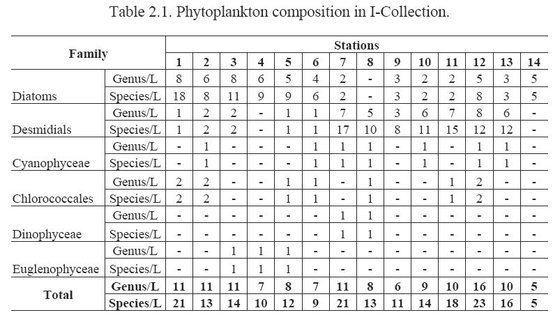
During first sampling, 100 species belonging to 37 genera were recorded. Of these 48 species belonged to Bacillariophyceae, 38 to Desmidials, 8 to Chlorococcales, 3 to Cyanophyceae, 2 to Euglenophyceae and one to Dinophyceae. Qualitative dominance of the phytoplankton in this collection was in the order of Bacillariophyceae > Desmidials > Chlorococcales > Cyanophyceae > Euglenophyceae > Dinophyceae. In this collection population of Desmidial member Staurastrum multispiniceps was highest (58,944/mL) in Station-7 (Muppane) of the reservoir. Among streams population of Bacillariophyceae member Synedra ulna was highest (35,136/mL) in Station-5 (Haridravathi main tributary).
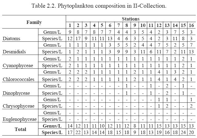
In this collection 117 species were recorded from 49 genera. Bacillariophyceae dominated with 49 species followed by Desmidials with 44; Chlorococcales with 14; Cyanophyceae with 5; Chrysophyceae with 3; and Dinophyceae with 2 species. Qualitative dominance was in the order of Bacillariophyceae > Desmidials > Chlorococcales > Cyanophyceae > Chrysophyceae > Dinophyceae. Among streams population of Gomphonema longiceps a Bacillariophycean was highest (21,568/mL) in Station-6 (Nandiholé - minor tributary), while among reservoir waters in Station-16 (Nittur), population of Dinobryon sertularia was highest (4752/mL).
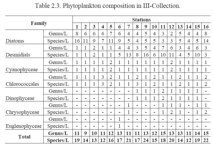
During this collection 110 species of phytoplankton belonging to 48 genera were recorded. Of these 41 species belonged to Bacillariophyceae, 39 to Desmidials, 16 to Chlorococcales, 9 to Cyanophyceae, 2 species each to Dinophyceae and Chrysophyceae and a single species to Euglenophyceae. Qualitative dominance was in the order of Bacillariophyceae > Desmidials > Chlorococcales > Cyanophyceae > Dinophyceae = Chrysophyceae > Euglenophyceae. Between both the waters of streams and reservoir, population of Navicula viridula was highest in Station-1 (Sharavathi-I, 27,728/mL) and Station-12 (Yenneholé, 5,648/mL).
The distribution pattern of phytoplankton was almost similar in all the collections. However, highest species were recorded in collection-II with 117 species and lowest in collection-I with 100 species. During collection-III, 110 species were recorded. From Tables 2.1, 2.2 and 2.3 it is clear that, in general in all the streams (Station 1-6 and 14) Bacillariophyceae (Diatoms) species dominated while in all the waters of reservoir (Station 7-13, 15, and 16) Desmidials predominated during all the collections. From the stationwise list of diatoms (Appendix-II) it is clear that, Gomphonema longiceps, Navicula viridula, Synedra ulna, Surirella ovata and many species of diatoms almost commonly occurred in all the streams. Similarly, species of desmids like Staurastrum limneticum, S. freemanii, S. multispiniceps, Arthrodesmus psilosporus, Triploceros gracile and Xanthedium perissacanthum almost commonly occurred in all the stations of the reservoir during all the three collections. Thus, the distribution pattern of diatoms and desmids indicates that species composition was almost similar in streams and reservoir waters during all the collections.
Cyanophyceae and Chlorophyceae members distributed uniformly in streams and reservoir waters, but Dinophyceae and Euglenophyceae were scantly distributed. Chrysophyceaen members did not occur during collection-I. During collection II and III, they were recorded from reservoir waters with 2 species of Dinobryon.
Bacillariophycean members Anomoeoneis sphaerophora, Gyrosigma attenuatum, G. gracile, Gomphonema lanceolatum, G. longiceps, Navicula viridula, Nitzschia obtusa, N. palea, Pinnularia lundii, P. maharashtrensis, Surirella ovata, Synedra acus and S. ulna were common to all the three collections. Desmidial members common to all the three collections were Arthrodesmus psilosporus, Closterium ehrenbergii, Cosmarium decoratum, Desmidium baileyi, Staurastrum limneticum, S. freemanii, S. multispinceps, S. peristephes, S. tohopekaligense and Triploceros gracile.
Chlorococcalean members Eudorina elegans, Muogeotia punctata, Pediastrum simplex, and Spirogyra rhizobrachialis were common in all the three collections. One Dinophycean member Ceratium hirundinella and one Cyanophycean member Microcystis aeruginosa were common in all the three collections.
Most of the other species of Diatoms, Desmids, Cyanophycean and Chlorococcalean were common to either collection-I and II or I and III or II and III indicating almost similar species composition in all the three collections.
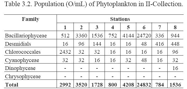
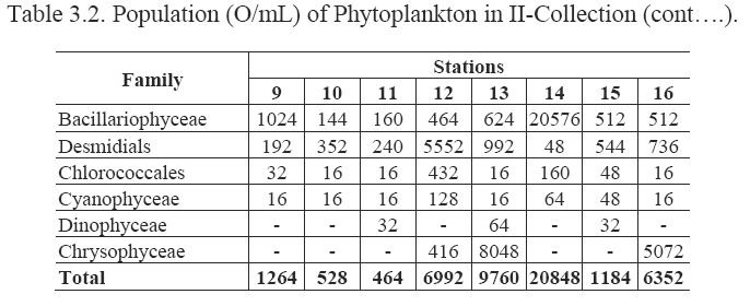
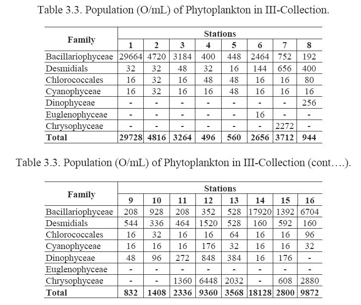
Generally blooms are formed under limnological conditions favoring high fertility at the water surface. Commonly a bloom of algae will form a scum on the surface or give distinct coloration to the water. Tables 3.1, 3.2 and 3.3 show the population of different algal groups in three collections. It is clear here that population of Bacillariophyceae (diatoms) is almost high in streams (Station 1-6 and 14) and that of desmids is in reservoir waters (Station 7-13, 15 and 16). However, none of the phytoplankton representing either Bacillariophyceae or Desmidials formed bloom during any of the three collections. Their individual population was not enough to form a scum on the surface to give distinct coloration to the water to form the algal bloom. However, Gomphonema longiceps predominated in Station-6 of collection - II, and Navicula viridula predominated in Station-14 of collection - II and Stations 1 and 14 of collection - III over all other phytoplankton. Population of Cyanophycean and Chlorococcalean species were very low. Dinophycean and Euglenophycean occurrence was scanty with negligible population. Chrysophycean species occurred only in II and III collections with dominance in some stations. Dinobryon sertularia dominated in Station-13 and 16 of collection - II and Stations 7, 11, 12 and 13 of collection - III.
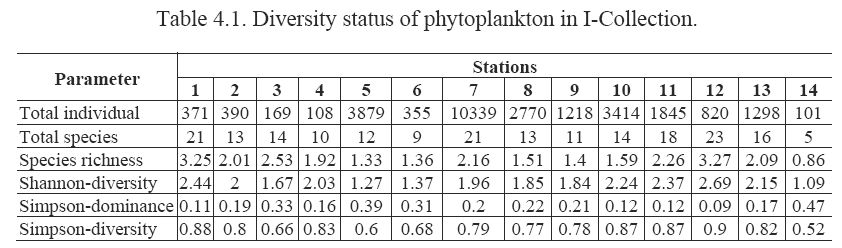
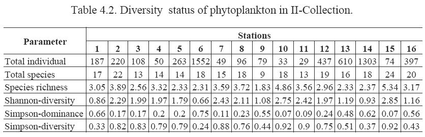
Tables 4.1, 4.2, and 4.3 reveal the diversity status of phytoplankton during I, II and III-collection. From these Tables it is clear that species diversity is not uniform in any station in any of the collections. This is mainly because of the non-uniformity in the occurrence of species and their population in these stations during all the collections.
From Table 4.1 it is clear that in general, total individuals are low in almost all the streams and high in almost all the waters of reservoir. Among all the stations total individuals are highest in Station-7 (10339) and lowest in Station-14 (101). Total species is high (23) in Station-12 with highest species richness (3.27) and Shannon diversity values (2.69), which is evident from the low Simpson dominance value and high evenness index value in Station-12. On the other hand in Station-14 species richness and Shannon diversity values are low (0.86 and 1.09 respectively) with high Simpson dominance (0.47) and low evenness index value (0.52).
From Table 4.2 it is clear that in general, in the waters of streams and reservoir total individuals are almost low as compared to collection - I. Total individuals are lowest (49) in Station-7 where it was high during I collection. Highest individuals were recorded in Station-6 (1552). Total species is high (24) in Station-15 with highest species richness (5.34) and Shannon diversity values (2.85), which is evident from the low Simpson dominance and high evenness index values. Total species is lowest (9) in Station-9 with lowest species richness (1.83) and almost lower Shannon diversity value (1.08). However, lowest (0.66) Shannon diversity is in Station-6 with highest Simpson dominance (0.75) and lowest evenness index values (0.24).
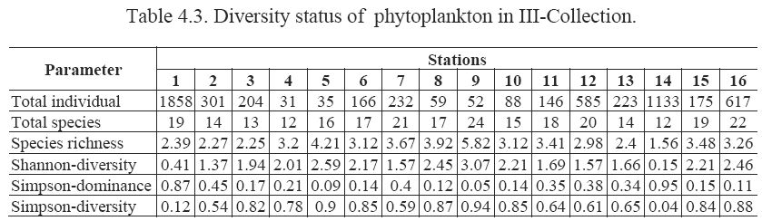
Table 4.3 indicates that the total individual value is highest (1858) in Station-1 and lowest (31) in Station-4. Total species is high (24) in Station-9 with highest species richness (5.82) and Shannon diversity (3.07) values. Lowest species richness value is in Station-14 (1.56) with lowest Shannon diversity (0.14), which is evident from the higher Simpson dominance (0.95) and lower evenness index (0.04) values. Vice versa was true with Station-9 where the Shannon diversity is high (3.07) with low Simpson dominance (0.05) and high evenness index values (0.94).
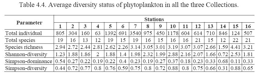
Table 4.4 reveals the average diversity status of phytoplankton of all the three collections. This table shows the highest population (3540) in Station-7 and lowest (63) in Station-4. Highest number of species is in Station-15 (22) with highest species richness (4.41) and highest Shannon diversity (2.53) values, which are indicated by low Simpson dominance (0.11) and high evenness index values (0.88). Lowest number of species is in Station-14 (12) with lowest species richness (1.59) and Shannon diversity (0.72) and with the highest Simpson-dominance (0.68) and lowest evenness index values (0.31). From Table 4.4 it is also clear that species richness and species diversity values are almost high in the waters of reservoir as compared to waters of streams. This might be due to the higher number of species (24 species) of Staurastrum, a desmidial member, which might have resulted in higher species diversity value in reservoir waters.
From the Tables 4.1, 4.2 and 4.3 it is clear that the Stations 7 and 1, which harboured highest and lowest total individuals respectively during I collection had almost low and high total individuals during II and III-collection. Similarly during collection II, Station-6, which harboured highest total individuals, showed lower population during I and III collection. This indicates that the growth and distribution patterns of phytoplankton are not uniform during all the collections. Further as compared to II and III-collections total individuals were high during I-collection. It might be because of the rains during the month of September just prior to I-collection during October, which might have added nutrients to the waters along with run-off water from surrounding catchment areas.
Thus, from the above discussion about species diversity of phytoplankton in various stations of streams and reservoir it is clear that diversity and species richness were not uniform in any stations during all the three collections. However, during I collection total population was highest in reservoir waters as compared to streams. It might be because of the higher nutrient load in stagnant waters of reservoir (due to rain just before I collection), which might have resulted in higher population of Desmidials in these waters. In general the requirement of dissolved oxygen for the growth of many diatom species is well documented. In the present study, in stream waters higher population of diatoms coincided with the higher dissolved oxygen, as oxygen is generally high in stream (flowing) waters compared to reservoir waters. The studies of Venkateshwarlu (1970) and Sheavly and Marshal (1989) who found that diatoms prefer well-aerated waters that are rich in dissolved oxygen is in support of present observation. Rao (1977) has observed dissolved oxygen favouring different species of diatoms, which is also found true for diatoms in the present study.
On the other hand reservoir waters showed lower species composition as well as population of diatoms. It may be due to their slight stagnant nature where dissolved oxygen content is less as compared to streams. However, in reservoir waters desmid species predominated. Generally, paucity of desmids is seen in the organically polluted waters. Waters supporting luxuriant growth of Desmidials have been found to be chemically distinct from those harbouring other members of algae (Hegde, 1985). The present study is on par with these observations, since desmids predominated in reservoir waters, which might have had lower organic pollution. On the other hand stream waters harboured lower desmid population indicating probable evidence of organic pollution as compared to the waters of reservoir.
In order to apply biological means of determining the trophic status Shannon and Weavers species diversity values, Nygaards phytoplankton Quotient and Palmers pollution indices of phytoplankton were calculated for the three collections of phytoplankton.
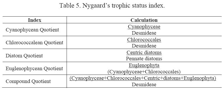
Nygaard (1949) has given ratios for plankton communities to decide the trophic status (Table 5).
For oligotrophic lakes of Denmark, investigated by Nygaard (1949), the values for Cyanophycean, Chlorococcales, Diatom, Eugleninae and Compound quotients were 0.0-0.4; 0.0-0.7; 0.0-0.0; 0.0-0.2 and 0.0-1.0 respectively. For eutrophic lakes the values of these quotients were 0.8-3.0; 0.7-3.5; 0.2-3.0; 0.0-0.2 and 2.0-8.75 respectively.
The 8 value indicates the absence of algal quotient representing groups in that collection. For example, for the calculation of Diatom Quotient both pinnate and centric diatoms should be present in a particular sample. Since centric diatoms were not collected in any of the three collections, the diatom quotient value is 8.
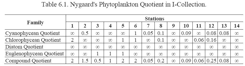
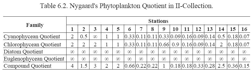
Table 6.1, 6.2 and 6.3 indicate the Nygaards phytoplankton quotient values. From Table 6.1 it is clear that almost all the values are very low to represent the eutrophic nature of the water. However, in some Stations (1, 3, 4, 5 and 6), the values were above the values given by Nygaard for oligotrophic waters. In Station-1, Chlorophycean and Compound quotient values, in Station-2 Compound quotient value, in Station-3 and 4 Euglenophycean quotient values, in Station-5 Chlorophycean, Euglenophycean and Compound quotient values and in Station-6 Cyanophycean, Chlorophycean and Compound quotient values exceeded the values given for oligotrophic nature of water. Interestingly all these Stations represents the streams. All the waters of reservoir show the oligotrophic nature as their quotient values are in between the values given by Nygaard for oligotrophic water. Similarly from Table 6.2 it is clear that, stream waters are slightly eutrophicated, as in Station-1 Cyanophycean, Chlorophycean and Compound quotient values, in Station-3 Chlorophycean and Compound quotient values and in Station-4 and 5 Cyanophycean and Chlorophycean quotient values exceeded the values given for oligotrophic nature of water. Similar to I-collection,the Nygaards phytoplankton values are in the range of oligotrophic nature in II-collection also, in all the reservoir waters.
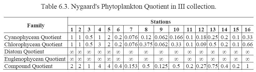
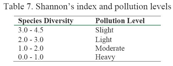
Table 6.3 almost confirms the findings of I and II-collections as the stream waters in III-collection are also eutrophic in nature. In Station-1 Cyanophycean, in Station-2 Chlorophycean, in Station-4 Cyanophycean, Chlorophycean and Compound quotient values and in Station-5 Cyanophycean, Chlorophycean and Compound quotient values have exceeded above the oligotrophic values. On the other hand waters of the reservoir are in between the values given for oligotrophic waters. Thus, it is clear from Nygaards pollution index that stream waters are slightly eutrophic in nature as compared to reservoir waters. Generally, waters of streams with rapid flow carry organic matter from the soil. In the present study, stream waters might have carried the organic matter from the soil and decomposed dried leaves of surrounding trees and resulted in the slight eutrophic nature of the waters. It is quite natural that in reservoir waters, the organic matter brought from runoff water during rains will settle down to the bottom in the winter season. This might be the reason for the lower organic pollution and oligotrophic nature of the reservoir waters as the collections of phytoplankton were made during the winter season. Biligrami (1988) has given the degrees of pollution based on the ranges of Shannon and Weiners species diversity (Table 7).
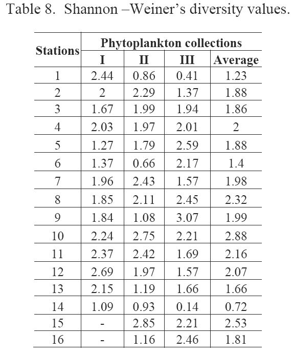
From Table 8 it is clear that in general species diversity values of almost all the stations are in the range of moderate or light pollution level. As per the pollution ranges given by Biligrami (1988), waters of Stations 1, 2, 4, 10, 11, 12 and 13 during I-collection, waters of Stations 2, 7, 8, 10, 11 and 15 during II-collection and waters of Stations 4, 5, 6, 8, 9, 10, 15 and 16 during III-collection show light pollution level with species diversity ranging between 2.0 3.0. While waters of Stations 3, 5, 6, 7, 8, 9 and 14 during I-collection, waters of Stations 3, 4, 5, 9, 12, 13 and 16 during II-collection and waters of Stations 2, 3, 7, 11, 12 and 13 during III-collection show moderate pollution level (Species diversity ranges between 1.0-2.0).
In II and III-collections stream waters show heavy pollution load in some stations. In II-collection waters of Stations 1, 6 and 14 and in III-collection waters of Stations 1 and 14 had heavy pollution load with the species diversity ranging between 0.0-1.0. Only the waters of Station-9 in III-collection had slight pollution level with the species diversity 3.07.
From the average species diversity values it is clear that almost all the waters of streams show moderate pollution level, while almost all the reservoir waters show light pollution level.
Thus, from the above discussion it is clear that waters of only Station-3 and 10 show uniformity i.e., moderate and light pollution level from I-collection to/and III-collection. Remaining waters during different collections show either light or moderate pollution level. Thus, the pollution level was not uniform in almost all the stations. It is in between the light and moderate pollution level with heavy pollution load in few stations of streams.
Another popular work on pollution aspect is of Palmer (1980) who has listed top 8 pollution tolerant genera, the Euglena, Oscillatoria, Chlamydomonas, Scenedesmus, Chlorella, Nitzschia, Navicula and Stigeoclonium and top 9 species Ankistrodesmus falcatus, Euglena viridis, Nitzschia palea, Oscillatoria limnosa, Oscillatoria tenuis, Pandorina morum, Scenedesmus quadricauda, Stegioclonium tenue and Synedra ulna. Further he has given the algal pollution indices developed for use in rating water samples for high or low organic pollution (based on 20 genera and 20 species). In analysis of a water sample, all of the 20 genera and species of algae that are present are recorded separately. An alga is called present if there are 50 or more individuals per ml. The pollution index factors of the algae present are then totalled. A score of 20 or more for a sample is taken as evidence of high organic pollution while a score of 15-19 is taken as probable evidence of high organic pollution. Low figures indicate that the organic pollution of the sample is not high.
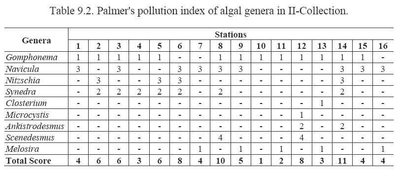
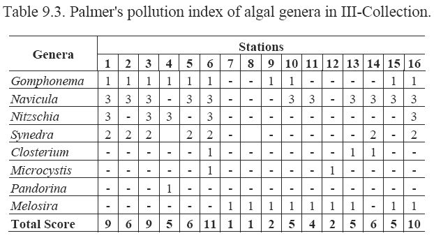
Tables 9.1, 9.2 and 9.3 reveal the Palmers genera index values. From Table 9.1, it is clear that all the stations with a score of less than 10 except Stations 5 and 13 are said to be less polluted. Stations 5 and 13 with score of 12 and 13 come nearer to the point of suspected pollution. Similarly, II collection and III-collection with scores less than 10 are indicating low organic pollution in all the stations (Tables 9.2 and 9.3). Thus, Palmers pollution index values of all the three collections are not exceeding the score given by Palmer (1960) for the high organic pollution or the probable evidence of organic pollution. Thus, the waters of all the stations during I, II and III-collections showed low organic pollution.
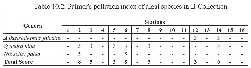
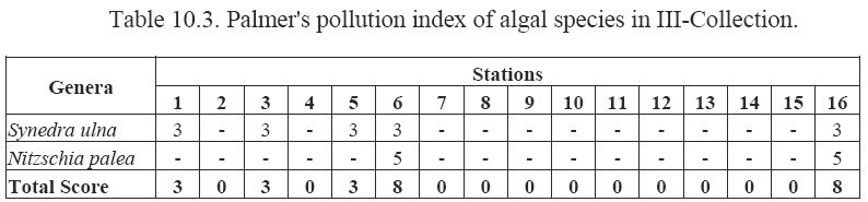
Out of the 20-algal species reported by Palmer, Synedra ulna and Nitzschia palea occurred in some of the stations of I and III-collections. In II-collection along with these two species Ankistrodesmus falcatus also occurred in some stations. Some other species like Pandorina morum and Scenedesmus quadricauda, even though occurred in some of the stations, are discarded due to their lower number (less than 50 per ml.).
Tables 10.1, 10.2 and 10.3 reveal the Palmers species index values. From these Tables it is clear that the total score of none of the stations of all the three collections exceeded the total score given by Palmer for high organic pollution or even probable high organic pollution. This indicates that waters of all the stations during all the three collections had low organic pollution.
From the species composition and growth of phytoplankton in various streams and reservoirs it is clear that waters of both streams and reservoir were below the level of high organic pollution. High pollution indicating organisms were very less in these aquatic ecosystems and the score of those present did not show the range of Palmers total score of high organic pollution.
By applying various pollution indices, it is clear that in general waters of both streams and reservoir are oligotrophic in nature, as there is no high organic pollution load in these waters. However, there is slight difference in the results of different pollution indices. Nygaards pollution index showed slight eutrophic quality for stream waters and oligotrophic for reservoir waters. While pollution index based on Shannon diversity showed no difference between streams and reservoir waters on the basis of oligotrophic and eutrophic natures. Results of this index indicated the slight eutrophication and oligotrophication in both the waters of streams and reservoir. Palmers genera as well as species pollution index showed no heavy load of organic pollution in any of the waters of both the streams and reservoir. According to Palmer (1980) Melosira islandica and species of Dinobryon are clean water indicators. The occurrence of Melosira islandica in stream waters and Dinobryon calciformis and D. sertularia in reservoir waters clearly indicate that both the waters are clean. Thus, there is no heavy organic pollution load in any of the waters of both streams as well as reservoir of Sharavathi River basin.
As all the stations of streams and reservoir are away from disturbances from cities and industries, presently there is no heavy organic pollution in these water-bodies. However, in future if there would be any pollutants like domestic and industrial wastes, there is a threat to the indigenous phytoplankton. Phytoplanktons are primary producers, on which many higher-level organisms like zooplankton and other aquatic higher animals are directly or indirectly dependent. So these contaminations may change their environment and affect the food chain. Due to this the organisms, which were in equilibrium with habitat earlier, will be unable to cope up with the changed environment and may disappear slowly.