Annexure A

Calibration of Hyperspectral data

L1B Emissive Calibration - The MODIS emissive calibration algorithm is designed to determine the at-aperture spectral radiance of the Earth scene with its associated uncertainties. Level 1A data is Earth-located raw sensor digital numbers and Level 1B data is Earth-located, calibrated data in physical units. The On-board Blackbody and Space View are used every scan to calibrate the emissive bands. The on-orbit emissive band MODIS calibration is a two point method which fits a nonlinear response by using pre-launch measurements [1].

Spectral Calibration - MODIS spectral band responses are well defined and stable. The MODIS bandpass filters were constructed with Ion Assisted Deposition (IAD), so the center wavelength for any of the solar reflecting spectral bands will not vary during the lifetime of MODIS. Spectral shifts have occurred for previous filter instruments going from ambient to vacuum. The spectroradiometric Calibration Assembly (SRCA) measures any prelaunch to on-orbit center wavelength shift. The SRCA has the capability of wavelength self-calibration for solar reflective bands [3].

Atmospheric Correction for MODIS

The MODIS atmospheric correction algorithm over land are applied to bands 1 – 7, centred at 648, 858, 470, 555, 1240, 1640 and 2130 nm. Previous operations have assumed a standard atmosphere with zero or constant aerosol loading and a uniform Lambertian surface. The MODIS algorithm relies on the modelling of atmospheric effects as described in the Second Simulation of the Satellite Signal in the Solar Spectrum Radiative Code (6S) [4] and is simplified in the MODIS code for operational application. The code is documented and includes simulation of the effects of the atmospheric point spread function and surface reflection directionality. Currently the 6S code is being used as a reference to test the correct implementation of the MODIS atmospheric correction algorithm [5].

The inclusion of specific bands for atmospheric sensing on the MODIS instrument provides for dynamic atmospheric correction and allows the estimation of surface directional reflectances in the MODIS land bands [6]. Data obtained from MODIS are free of clouds, atmospheric contamination, and angular view and illumination effects. Rectification has posed particular difficulties for AVHRR processing in producing composited images, analyzing time trajectories of land surface data, and comparing data from multiple time periods to assess change. These problems are significantly reduced with the in-flight navigation capabilities of MODIS. Geolocation error estimates of MODIS, combined with the growth of pixel size with scan angle, provide an effective pixel size close to 1-km using the 500-m and 250-m land bands as inputs [7].

Description of PCA

Fundamentals of PCA

Principal component analysis is an analytical procedure for transforming one set of variates into another set of component variates having the following properties [8]:

•  They are linear functions of the original variates.

•  They are orthogonal, i.e., independent of each other.

•  The total variation among them is equal to the total variation in the original variates, consequently, information concerning differences among the observed variates is not lost in transformation unless the lower-order PCs are simply discarded.

•  The variance associated with each component decreases in order, the first variate will account for the largest possible proportion of the total variation, the second will account for the largest proportion of the remainder, and so forth.

(ii) PCA Operational Sequence

The important mathematical operational sequences of PCA that represents only one aspect of the analysis is as follows:

•  Selection of the preliminary variables

•  Determination of either the variance-covariance or the correlation matrix

•  Calculation of the above matrix

•  Determination of the eigenvalues and eigenvectors of the matrix

•  Formation of the new coordinate system, using the eigenvectors and

•  Interpretation of derived components.

The primary step of selecting the preliminary variable is extremely significant. These variables should be quantitative characters, and preferably be measured on a continuous scale, although many discrete variables adequately approximate continuous variables [9]. Consequently, the next step involves the use of either the variance-covariance matrix or the correlation matrix. Normally, if all units are of the same scale (e.g., all units of length), the use of the variance-covariance matrix is recommended. Use of the variance-covariance matrix has the greatest statistical appeal because the sampling theory is less complex than the others [10]. However, if the units are mixed (e.g., length, volume, weight), normalization becomes important and the correlation matrix is used. The linear transformation of p original variants into p “artificial” variates is the third step involved in the transformation. This is the mathematical equivalent of determining the eigenvectors and related eigenvalues of a variance-covariance or of a correlation matrix.

Conceptually, this requires the extraction of common variables (i.e., the eigenvectors) and their variances (i.e., eigenvalues) from the variance-covariance or correlation matrix. A simplistic development of the mathematical derivation of eigenvectors and eigenvalues can be found in [11].

(iii) Mathematical Description of PCA

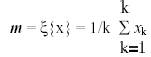
Consider a multispectral space with a large number of pixels plotted in it. Each pixel is described by its appropriate vector x. The mean position of the pixels in the space is defined by the expected value of the pixel vector x , according to

------------------------ (equation 2.3)

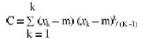
where, m is the mean pixel vector and the x_k are the individual pixel vectors of total number k; is the expectation operator. While the mean vector is useful to define the average or expected position of the pixels in multispectral vector space, it is of value to have available a means by which their scatter or spread is described. The covariance matrix is defined as

------------------ (equation 2.4 )

in whic h the superscript ‘t' denotes vector response. An unbiased estimate of the covariance matrix C is given by

-----------------------(equation 2.5)

where,

K = Total number of pixels in an image

m= total number of bands used in the analysis

The covariance matrix is one of the most important mathematical concepts in the analysis of multispectral remote sensing data. If the correlation matrix is to be used, each entry in C should be divided by the product of the standard deviation of the features represented by the corresponding row and column (i.e., the covariance between image in band 1 and image in band 2) in the matrix C, then the corresponding correlation r₁₂ is obtained by

-----------------------------(equation 2.6)

where, , are the standard deviations of band 1 and band 2, respectively. Correlation for the other entries can also be found in a similar manner. The next step is calculation of the eigenvalues and eigenvectors of the matrix C. It is determined by solving the following equations

----------------------------(equation 2.7)

Where A _i= (a₁ , a₂ , ...a_m) t is the eigenvector corresponding to the eigenvalue m is the feature space dimension and I is the identity matrix (i.e., a matrix with diagonal entries set to 1 and off-diagonal entries are set to 0).

All the eigenvalues ¸ can be determined by solving

------------------------- (equation 2.8)

And finally the new coordinate system is formed by normalized eigenvectors of the variance -covariance (or correlation) matrix .The mapping location f_i of each pixel X = (x₁ , x₂ , x₃...x_k ) on the i th principal component is given by:

f_i = X * A_i = x₁ * a₁ + x₂ * a₂ + ... + x_k * a_k--------------------------(equation 2.9)

The atmospheric correction for MODIS data in heterogeneous ground conditions has been addressed by several researchers [12], [13] and [14]. The atmospheric correction approach adopted by MODIS is to assume that the signal received by the satellite is a combination of the reflectance of the target pixel and reflectances from the surrounding pixels, each weighted by their distance from the target. Because the apparent signal at the top-of–the-atmosphere (TOA) comes from the target and adjacent pixels, this effect is called the adjacency effect. The correction involves inverting the linear combination of reflectances to solve for the reflectance of the target pixel [5].