|
Results |
Land use analysis: Classified land uses during 1977, 1992, 2000, 2010 and 2014 are shown in fig.4. Analyses of the temporal remote sensing data reveals an increase in built up area of 262% (during 1977 to 1992), 211% (during 1992 to 2000), 250% (2000 to 2010) and 149% (2010 to 2014). Similarly, the extent of other category (including the cultivation lands, barren lands, open lands, etc.) has drastically increased from 5% in 1977 to 65% in 2010 showing 3000% growth during the last four decades with 70 % decline of vegetation cover. LU analyses (Table 4) reveal that urbanization has led to the loss of arable land, decline in natural vegetation cover as well as habitat destruction. Accuracy assessment and kappa statistics were calculated, overall accuracy ranged from 85% - 95% and kappa values ranged from 0.84 – 0.94
Table 4. Land use of Bhopal during 1977 to 2014.
Year |
Urban (%) |
Vegetation (%) |
Water (%) |
Others (%) |
1977 |
0.35 |
92.04 |
2.15 |
5.45 |
1992 |
0.93 |
66.52 |
2.38 |
30.17 |
2000 |
1.96 |
37.25 |
2.14 |
58.65 |
2010 |
4.90 |
28.02 |
1.82 |
65.26 |
2014 |
7.31 |
21.77 |
2.09 |
68.83 |
3.3.1. Density gradient analysis
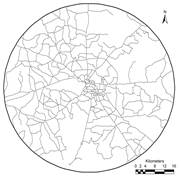
Study area was divided into concentric incrementing circles of 1 km radius (with respect to centroid or central business district) in each zone.
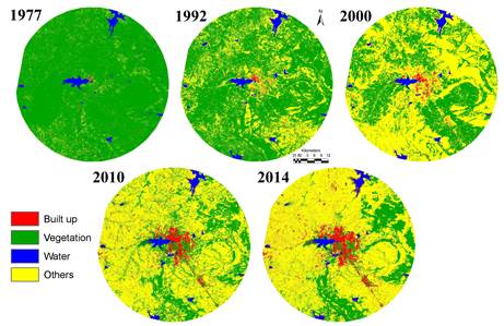
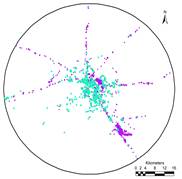
Fig. 4. Land use changes from 1977 – 2014.

Fig. 5. Gradient analysis of Bhopal Built-up density circle (urban area/ total area) - and zonewise.
The urban density computed for each gradient of respective zones for the period 1977 to 2014 is given in Figure 6. This highlights the radial pattern of urbanization with the concentrated growth closer to the central business district and minimal growth in 1977. Bhopal grew intensely in the NW and SE zones in 1977-1992 due to the industrialization in the region. The industrial layouts came up in SE and housing colonies in NW and NE and urban sprawl was noticed in others parts of the Bhopal. This phenomenon intensified with development of industrial sectors in SE and NW during post 2000.
The analysis showed that Bhopal grew radially from 1973 to 2014 indicating that the urbanisation has intensified from the city centre and reached the periphery of Bhopal. Annual growth of Madhya Pradesh is one of the highest in the country as Gross domestic state product is 11.68% in the 2014-2015.
After reorganization in 1956 and naming Bhopal as capital of state of Madhya Pradesh, Planners looked at building new Bhopal city away from the so called city centre, which remained planned until late 1990’s, wherein Industrialization took over developing the Bhopal Metropolitan Region that encompasses regions of Rajgarh, Raisen and Vidisha. Bhopal city enjoys the development of towns that are known as market towns established in late 90’s named Berasia, Vidisha, Raisen, Sehore, Budhni, Itarsi. Fact that the planners have visualized good connectivity with road infrastructure but have failed to provide regional connectivity to the national mainstream, due to which we see huge developments in these regions in terms of sprawl
Prior to industrial advent in Bhopal, city had few planned industrial colonies such as BHEL in the newer planned city regions, and connected the old city. With advent of industries in 1990’s Bhopal started expansion towards north east specifically towards Vidisha. This pattern changed in late 90’s and with industrial colonies in southern regions Bhopal expanded and sprawled towards south east near Mandideep and shobhapur. which has continued over the next decade with sprawl is around the airport, railway cantonment. Though planners had visualized growth of Bhopal, but huge rampant urban sprawl was not understood.
3.3.2. Spatial patterns of urbanisation
Spatial patterns of urban growth were analysed zone wise for each circle of 1 km radius considering temporal land use information using five landscape level metrics and are discussed below:
a). Number of patches (NP): Figure 6 illustrates the temporal dynamics of number of patches. In the year 1977 inner circles close to CBD (1-7) have patches close to 1 indicative of fact that these regions are in the state of clumped growth which are common in NE, SE and SW directions. In NW direction, the core is fragmented showing that these regions are dominated by all classes. In all directions, there are fragmented buffer regions with number of patches ranging from 10 – 40 except south west which has seen higher fragmentation in 1977. But in 2010 and 2014 the buffer regions have become more fragmented with patches ranging from 280-518, which shows that the regions are under the pressure of urban sprawl and fragments of urban area have increased which in turn has led to dominance of urban in the region. All directions show fragmented growth, with higher fragmentation ~500 -800 fragments in North West region in the buffer zone.
b). Total Edge (TE)- During 1977 the edges were smaller, as the urban patch was rare and concentrated in landscape, but post 2000 and in 2014 there are larger edges, which indicate that the urban area is continuous. This phenomenon is true in the city boundary, but the buffer region patches are yet fragmented and non-continuous. In 2014, TE steadily increase in the outer circle showing further fragmentations in all directions with the highest fragments in NW zone indicating that these regions are dominated by all classes. South West zone had minimal fragmentation but a concentrated growth with less number of edges.
c). Normalized Landscape Shape Index (NLSI). Results depicts fragmented landscape during post 2000 and in 2014, the landscape is highly fragmented in the buffer region. In 1977, the lower value of NLSI in all three directions except NW, with regular shape (Circle, Square) in the inner circle near to CBD (1-7). NW direction close to city centre (1-7) show fragments ensuring core is dominance by all classes. In 2014, the NLSI show almost similar value for the core area (1-7) in all the direction indicating the fact that these regions are in the verge of forming a single urban patch and North East is the direction that is severely affected by urbanisation indicating irregular shape at the centre. In SW direction (circle 7 and 8) having 0 value of NLSI showing single maximally aggregated patch completely dominated by water cover. The result also assures fragmented growth in 2014 near the CBD as compared to 1977 indicating irregular shape at the centre. NLSI demarcates that the urban area is almost clumped in all direction and all gradients especially in NW and SE direction. It shows a small degree of fragmentation in the buffer regions in SW direction. The core area is in the process of becoming maximally uniform shape (such as square, circle etc.) in all directions.
d). Clumpiness index (CLUMPY) represents the similar trend of compact growth at the center of the city which gradually decreases towards outer rings indicating the urban agglomeration at centre and phenomena of sprawl at the outskirts in 2014. Figure 7 with the Clumpy values of 1 at core areas (in 1977) indicates of a clumped growth in all direction except North West. In 2010, the value of clumpy index gradually decreased in the inner circle (1-7) showing that the CBD is under the pressure of urbanization with more aggregated growth in SE. NW in 2010 has lowest value of clumpy showing higher fragmentation in the buffer region. The buffer region has become more fragmented in North West Direction by 2014 followed by South East shows that the regions is under the pressure of urban sprawl and fragments of urban area have increased which in turn has led to dominance of urban in the region.
The analysis of spatial patterns using landscape metrics highlight of compact growth with intense urbanisation in 2010. Central areas have a high level of spatial accumulation and corresponding land uses, such as in the CBD, while peripheral areas have lower levels of accumulation. Unplanned concentrated growth or intensified developmental activities in a region has telling influences on natural resources (disappearance of open spaces – parks), enhanced pollution levels and also changes in the local climate.
3.3.3. CA Modelling (validation and prediction)
Land use [LU] transitions were calculated to predict land use for the year 2014, using Markov chain based on LU of 2000 and 2010. CA hexagonal filter (5x5) was used to generate spatially explicit contiguity weightage factor to change the state of the cell based on neighbourhoods. Predicted land uses of 2014 was compared with actual land uses of 2014 classified based on remote sensing data with field data. Results reveal that predicted and actual land uses are in conformity with kappa value of 0.83 and overall accuracy being 86% (Table 5). With the knowledge of 2000, 2010 and 2014, LU is predicted for 2018 and 2022 (Fig. 8). This prediction has been done considering water bodies as constraint and assumed to remain constant over all time frames. Table 6 tabulates predicted land use statistics of Bhopal city for the year 2018 and 2022.
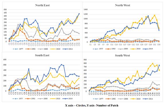
Fig. 6. Analysis of number of patches in the study region.

Fig. 7. Analysis of Clumpiness in the study region.
The main concentration will be mainly in the vicinity of NH12 and proposed outer ring road. Predicted land use also indicates densification of urban utilities near the Raja-Bhoj airport and surroundings. Further an exuberant increase in the urban paved surface growth due to industrial areas in south east and North West. The results also indicated the growth of suburban towns such as Vidhyanagar, Mandideep, Avadhpuri, Shobhapur, Obaidullganj, Bharkeda, Jharkheda, Toomda and Thuna Kalan [Fig. 9] with urban intensification at the core area. The predicted urban area is expected to increase by 50% in 2018 and 121% by 2022 compared to 2014. This highlights the need for appropriate infrastructure and basic amenities to cope up with the visualized growth and minimize drudgery to the common public. Since the model doesn’t consider the factors(s)/ Agents of growth it may be noted that few regions especially the core and regions in Obaidullganj and Shobhapur that are major regions of today’s growth have not shown urbanisation reason that can be attributes is mainly due to neighbourhood effect. Regions on the south and east that have new developments in today’s context have been omitted since previous maps that were used for training and prediction has no reference of today’s growth. Overall, Ca-Markov underestimated the land use for 2014, which can be avoided using drivers of urban growth through Agent Based model. Factors that express influence and weights were obtained through fuzzy –AHP, which were used in ABM. Validation was performed show kappa of 0.93 and overall accuracy of 93.5%. Figure 10 shows examples of select factor(s) considered for ABM. Figure 11 shows the results of Fuzzy – AHP based agent based urban model for 2014, 2018 and 2022 and land use details are tabulated in Table 5 (for 2014) and 7 (for 2018 and 2022). ABM based prediction for built-up was comparable to the actual values (agreement greater than 99%). ABM could also bring out the major regions of growth such as Toomda and Sehore that are in the influence of urbanisation recently. Clearly ABM bought out region specific growth with different agents. It can be noted that infrastructure such as road and rail are good in Bhopal and we could understand the urban development would happen in these corridors along with developments in industrial location. Roads, basic amenities like schools, hospital and job locations were main factors that were influencing urban growth in these regions. It may be essential to plan these basic amenities before planning further developments towards Indore, Sehore, and Obaidullganj.
Table 5. Comparison of predicted land use (2014) with actual land use of 2014
Class year |
Built-up area (%) |
Vegetation |
Water |
Others |
2014 classified |
7.31 |
21.77 |
2.09 |
68.83 |
2014 predicted (CA Markov) |
5.71 |
33.93 |
1.73 |
58.63 |
2014 predicted (ABM) |
7.02 |
18.84 |
2.12 |
71.98 |
Overall accuracy = 0.82 K location = 0.84 K standard = 0.73 (CA-Markov) |
||||
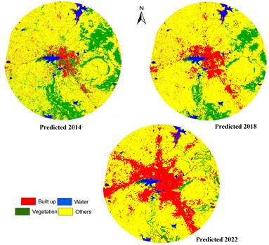
Fig. 8. Predicted growth of Bhopal using CA-Markov.
Table 6. Predicted Land use statistics of Bhopal using CA-Markov
Class year |
Built-up area (%) |
Vegetation |
Water |
Others |
2018 Predicted |
10.94 |
24.11 |
2.35 |
62.60 |
2022 Predicted |
16.14 |
28.03 |
2.52 |
53.31 |
Fig. 9: Probable urban growth locations
|
|
Fig. 10: Example of Factor(s) considered for the analysis |
|
|
|
|
|
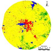

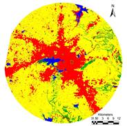

Fig. 11: Modelling urban growth considering Agents (ABM)
Table 7. Predicted Land use statistics of Bhopal using Agent based model.
Class year |
Built-up (%) |
Vegetation |
Water |
Others |
(%) |
(%) |
(%) |
||
2018 Predicted |
11.51 |
11.1 |
2.41 |
74.99 |
2022 Predicted |
25.09 |
4.71 |
2.12 |
69.09 |