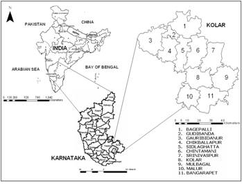
Study Area: The Kolar district in Karnataka State, India, located in the southern plain regions (semi arid agro-climatic zone) and extending over an area of 8238 km² between 77°21’ to 78°35’ E and 12°46’ to 13°58’ N, was chosen for this study (Fig. 1). The field data, remote sensing data, socio-economic data and other relevant information were available as a part of ongoing ecological studies in the region. Kolar is divided into 11 taluks for administration purposes. Rainfall occurs mainly during southwest and northeast monsoon seasons. The average population density of the district is about 209 persons/km². Kolar belongs to the semi arid zone of Karnataka. In the semi arid zone apart from the year-to-year fluctuations in the total seasonal rainfall, there are also large variations in time of beginning of rainfall, adequate for sowing as well as in the distribution of drought periods within the crop-growing season. Out of about 2800 sq. km. of land under cultivation, 35% is under well and tank irrigations. There are about 951 big tanks and 2934 small tanks in the district. The district is devoid of significant perennial surface water resources. The ground water potential is also known to be limited. The terrain has a high runoff due to limited vegetation cover, contributing to erosion of the top productive soil layer and leading to poor crop yield. The study area is mainly dominated by agricultural land, built up (urban/rural), evergreen/semi-evergreen forest, plantations/ orchards, waste lands and water bodies.

Fig. 1: Study area – Kolar district, Karnataka State, India

Data : The data sets needed to develop the vegetation database included village maps, Survey of India toposheets (1:50,000, 1:250,000), IRS (Indian Remote Sensing Satellite) images (multispectral) and information from field surveys (training data) using global positioning system (GPS).

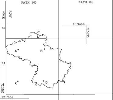
IRS - 1C/D LISS-III MSS (Multi Spectral Scanner) data in 3 bands (G, R and NIR, 0.52 to 0.86 μm) with a spatial resolution of 23.5 m were purchased from NRSA (National Remote Sensing Agency), Hyderabad.

Fig. 2: Kolar district with IRS 1C/1D Path-Row details

Land Cover Analysis : Land cover analysis was done using different slope and distance based vegetation indices (VI’s). Vegetation Indices (VI) are used to quantify the abundance and vigour of vegetation imaged by multispectral sensors. The differential reflectances in multispectral bands provide a means of monitoring density and vigour of green vegetation growth using the spectral reflectivity of solar radiation. Green leaves commonly have larger reflectances in the near infrared than in the visible range. As the leaves come under water stress, become diseased or die back, they become more yellow and reflect significantly less in the near infrared range. Clouds, water, and snow have larger reflectances in the visible than in the near infrared while the difference is almost zero for rock and bare soil. This helps in identifying observed physical cover including vegetation (natural or planted). VI is computed based on the data grabbed by space borne sensors in the range 0.6-0.7 (red band) and 0.7-0.9 (Near-IR band), which helps in delineating the area under vegetation and non-vegetation areas.  Broadly VI’s are categorized as Slope based VI and Distance based VI, which are discussed next.

Slope Based VI’s : Slope based VI’s computations are done using data acquired in visible red and near IR bands. These values indicate both the status and abundance of green vegetation cover and biomass. This is the first level of classification and aid in delineating areas under vegetation from non-vegetation.

1. Ratio : RATIO vegetation indices (Rose J.W. Jr et al, 1973) separate green vegetation from soil background by dividing the reflectance values contained in the near IR band (NIR) by those contained in the red band (R).
   
   

   Ratio  = NIR / RED

   (1)

   This clearly shows the contrast between the red and infrared bands for vegetated pixels with high index values being produced by combinations of low red (because of absorption by chlorophyll) and high infrared (as a result of leaf structure) reflectance. Ratio value less than one is taken as non-vegetation while ratio value greater than one is considered as vegetation. The major draw back in this method is the division by zero. Pixel value of zero in red band will give the infinite ratio value. To avoid this situation Normalized Difference Vegetation Index (NDVI) is computed.

2. Normalized Difference Vegetation Index (NDVI) : NDVI overcomes the problem of Ratio method  (i.e. division by zero). It was introduced in order to produce a spectral VI that separates green vegetation from its background soil brightness using IRS 1C MSS digital data (Rose J.W. Jr et al, 1973, Rose J.W. Jr et al, 1974) and is given by,
   
   

   NDVI = (NIR - RED)/(NIR + RED)

   (2)

   It separates green vegetation from its background soil brightness and retains the ability to minimize topographic effects while producing a linear measurement scale ranging from –1 to +1 with 0 representing no vegetation. This difference is sensitive to the presence of vegetation, since green vegetation usually decreases the signal in the red due to chlorophyll absorption and increases the signal in the NIR wavelength. It is preferred to the simple index for global vegetation monitoring because the NDVI helps compensate for changing illumination conditions, surface slope, aspect, and other extraneous factors. NDVI variation could be attributed to several vegetation phenomena ranging from vegetation seasonal dynamics at global and continental scales to tropical forest clearance, leaf area index measurement, biomass estimation, percentage ground cover determination, and photosynthetically active radiation estimation. These could be useful in various models to study photosynthesis, carbon budgets, water balance, and related processes. Vegetation NDVI typically ranges from 0.1 up to 0.6, with higher values associated with greater density and greenness of the plant canopy. Surrounding soil and rock values are close to zero while the differential for water bodies such as rivers and dams have the opposite trend to vegetation and the index is negative

3. Ratio Vegetation Index (RVI) : The ratio vegetation index is the reverse of the standard simple ratio (Richerdson A.J et al, 1977),
   
   

   RVI= RED/NIR

   (3)

   The range for RVI extends from 0 to infinity. The ratio value less than one is taken as vegetation while value greater then one is considered as non-vegetation area.

4. Normalized ratio Vegetation Indexes (NRVI) : Normalized ratio vegetation index is a modification of the RVI (Baret F et al, 1991) where the result of RVI-1 is normalized over RVI+1.
   
   

   NRVI=(RVI-1)/(RVI+1)

   (4)

   This normalization is similar in effect to that of NDVI, i.e it reduces topographic, illumination and atmospheric effects and it creates a statistically desirable normal distribution. Ratio value less than 0.0 indicates vegetation area while greater than 0.0 values represents non-vegetation.

5. Transformed Vegetation Index (TVI) : TVI is a modified version of NDVI to avoid operating with negative NDVI values (Deering, D.W et al, 1975). Adding 0.50 to NDVI value and taking the square root of the result computes TVI value. The calculation of the square root is intended to correct NDVI values approximate a Poisson distribution and introduce a normal distribution.
   
   

   TVI = √(NIR-RED/NIR+RED)  + 0.5

   (5)

   However negative values still exist for values less than – 0.5 NDVI. There is no technical difference between NDVI and TVI in terms of image output or active vegetation detection. Ratio values less than 0.71 is taken as non-vegetation and value greater than 0.71 gives the vegetation area.

6. Corrected Transformed Vegetation Index (CTVI) : CTVI suppresses the negative values in NDVI and TVI (Perry Charles R Jr. and Lautenschlager Lyle F. 1984). Adding a constant of 0.5 to all NDVI values does not always eliminate all negative values as NDVI values ranges from – one to + one. Values that are lower than –0.50 will leave small negative values after the addition operation. Thus CTVI is intended to resolve this situation by dividing (NDVI+0.50) by its absolute value ABS (NDVI + 0.50) and multiplying the result by the square root of the absolute value (SQRT[ABS(NDVI + 0.50)]).
   
   

   CTVI=(NDVI + 0.5)/Abs(NDVI+0.5) * √ Abs(NDVI+0.5)

   (6)

   The correction is applied in a uniform manner, the out put image using CTVI should have no difference with the initial NDVI image or the TVI whenever TVI properly carries out the square root operation. The correction is intended to eliminate negative values and generate a VI image that is similar to, if not better than, the NDVI. Ratio value less than 0.71 is taken as non-vegetation and value grater than 0.71 gives the vegetation area.

7. Thiam’s Transformed Vegetation Index (TTVI) : The CTVI image is very noisy due to an overestimation of the greenness, which can be avoided by ignoring the first term of the CTVI, and it provides the better results (Thiam A.K, 1997) This is done by simply taking the square root of the absolute values of the NDVI in the original TVI expression to have a new VI called as TTVI. It can be defined as:
   
   

   TTVI = √abs{(NIR-RED)/(NIR+RED)}+ 0.5

   (7)

   Ratio value less than 0.71 is taken as non-vegetation and value greater than 0.71 gives the vegetation area.

Distance Based VI’s: The main objective of the distance based vegetation index is to cancel the effect of soil brightness in cases where vegetation is sparse and pixels contain a mixture of green vegetation and soil back ground. This is particularly important in arid and semi-arid environment such as Kolar district of Karnataka.

Distance-based Vegetation indices are evaluated on the basis of soil line intercept concept. The soil line is a hypothetical line in spectral space that describes the variation in the spectrum of bare soil in the image. The soil line represents a description of the typical signatures of soils in red/near-infrared bi-spectral plot. It is obtained through linear regression of the infrared band against the red band for sample of bare soil pixels. Pixels falling near the soil line are assumed to be soils while those far away are assumed to be vegetation. Distance based VI’s using the soil line require the slope (b) and intercept (a) of the line as inputs to the calculation. Unfortunately there has been a remarkable inconsistency in the logic with which this soil line has been developed for specific VI’s. For evaluating PVI2, PVI3, TSAVI1, TSAVI2, it requires red band as independent variable for the regression while for evaluating PVI, PVI1, DVI, WDVI and MSAVI requires infrared band as independent variable for regression.

The soil line calculated for a set of soil pixels through regression analysis taking red band and infrared band as independent variable respectively and the relation is given as:

Y1=0.841333x + 10.781234 (red band independent variable)	(8)
Y2=0.985684x + 9.501355(infra-red band as independent variable)	(9)

The procedure requires that a set of bare soil pixels as a Boolean mask (value ‘one’ is assigned to pixels representing soil while ‘0’ for others). Analysis is done by regressing the red band against infrared band and vice versa. This provides slope and intercept of soil line.

8. Perpendicular Vegetation Index (PVI) : PVI uses the perpendicular distance from each pixel co-ordinate to the soil line and this was derived to define vegetation and non-vegetation for arid and semi arid region (Richerdson A.J et al, 1977). The pixels, which are close to soil line, are considered as non-vegetation while pixels, which are away from soil lines, represent vegetation. PVI values for data taken at different dates require an atmospheric correction of data, as PVI is quite sensitive to atmospheric variations.  This can be defined as:
   
   

   PVI= sin(a)NIR - cos(a)red

   (10)

   Where, a: Angle between the soil line and the NIR axis.
   

   PVI=√(x2 – x1)2 + (y2-y1)2

   (11)

   Where, (x₁, y₁) is the co-ordinate of the pixel and (x₂, y₂) is the coordinate of soil line point that is perpendicular to pixel co-ordinate.

   Perpendicular distance less then seven is taken as non-vegetation area while greater than seven is taken as vegetation area.

9. PVI1 : It was noticed that original PVI equation is computationally intensive and does not discriminate between pixels that fall to the right or left of the soil line (i.e. water from vegetation). Given the spectral response pattern of vegetation in which the infrared reflectance is higher than the red reflectance, all vegetation pixels will fall to the right of the soil line. In some cases a pixel representing non-vegetation (e.g. water) may be equally far from the soil line but it will fall left side of the soil line.

   In PVI the water pixel will be assigned a high vegetation index value. PVI1 assigns negative values to those pixels, which can be delineated from vegetation. The mathematical equation for PVI1 (Perry Charles R Jr. and Lautenschlager Lyle F. 1984) is written as,
   

   PVI1 =  (bNIR – RED +a) / √(b2+1)

   (12)

   Where, NIR: reflectance in the near infrared band, RED: reflectance in the red band, a: intercept of the soil line, b: slope of the soil line.
   
   Infrared band is taken as the independent variable and the red band as dependent variable for regression analysis. Perpendicular distance less then 6.5 is taken as non-vegetation area while greater than 6.5 is taken as vegetation area.

10. PVI2 : In PVI2, Red band is taken as independent variable over infrared dependent variable for regression analysis (Bannari et al, 1996) given importance to the red band with the intercept of soil line. Mathematically PVI2 can be represented as,
    
    

    PVI2 =  √{(NIR – a * RED +b) / √(a2+1)}

    (13)

    Where, a: intercept of the soil line, b: slope of the soil line.
    Here, pixels having less than –95.0 are grouped as non-vegetation area.

11. PVI3 : PVI3 is improved version of PVI, where red band is taken as independent variable on regression analysis and special attention was given to avoid the negative results (Qi, J. et al, 1994). PVI3 can be defined as,
    
    

    PVI3= apNIR – bpRED

    (14)

    Where, a: intercept of the soil line, b: slope of the soil line, pNRI: reflectance in the near infrared band, pRED: reflectance in the visible red band.

12. Difference Vegetation Index (DVI) : DVI weigh up the near-infrared band by the slope of the soil line (Richerdson A.J et al, 1977) and is given as :
    
    

    DVI= gNIR – RED

    (15)

    Where, g: the slope of the soil line.
    Similar to the PVI1, with the DVI, a value of zero indicates bare soil, values less than zero indicate non vegetation and greater than zero indicates vegetation.

13. Ashburn Vegetation Index (AVI) : AVI (Ashburn P, 1978) is presented as a measure of growing green vegetation. Scaling factor is required for evaluating AVI. For IRS 1C data scaling factor of one was chosen, as all bands are seven -bit. AVI can be represented as,
    
    

    AVI= sNIR – RED

    (16)

    Where, s: scaling factor.
    AVI was evaluated for Kolar district using scaling factor as one for eight-bit MSS data set.

    Soil noise : Soil reflectance spectra depend on type of soil.  The vegetation indices computed earlier assume that there is a soil line, where there is a single slope in red-NIR space. However, it is often the case that there are soils with different red-NIR slopes in a single image.  Also, if the assumption about the isovegetation line   (parallel or intercepting at the origin) is not exactly right, changes in soil moisture (which move along isovegetation lines) will give incorrect answers for the vegetation index.  The problem of soil noise is most acute when vegetation cover is low. The following groups of indices like SAVI, TSAVI1, TSAVI2, MSAVI1, MSAVI2 attempt to reduce soil noise by altering the behaviour of the isovegetation lines.  All of them are ratio-based, and the way they attempt to reduce soil noise is by shifting the place where the isovegetation lines meet. These indices reduce soil noise at the cost of decreasing the dynamic range of the index.  These indices are slightly less sensitive to changes in vegetation cover than NDVI (but more sensitive than PVI) at low levels of vegetation cover.  These indices are also more sensitive to atmospheric variations than NDVI (but less so than PVI).     
    

14. Soil-adjusted Vegetation Index (SAVI) : SAVI is intended to minimize the effects of soil background on the vegetation signal by incorporating a constant soil adjustment factor L in the denominator of the NDVI equation (Huete A.R ,1988). L varies with the reflectance characteristics of soil (i.e. color and brightness). The L factor chosen depends on the density of the vegetation. For very low vegetation L factor can be taken as one while for intermediate it can be taken as 0.5 and for high density 0.25. The best L value to select is where the difference between SAVI values for dark and light soil is minimal. For L=0, SAVI equals NDVI. For L=100, SAVI approximates PVI. Mathematically SAVI is defined as,
    
    

    SAVI = {(NIR - RED) /( NIR+RED+ L)}*(1+L)

    (17)

    Where, NIR: near-infrared band, RED: visible red band, L: soil adjustment factor.

    Multiplicative term (1+L) present in SAVI (and MSAVI) is responsible for vegetation indices to vary from – one to + one. This is done so that both vegetation indices reduce to NDVI when the adjustment factor L goes to zero. Soil adjustment factor (L) of 0.5 was considered for Kolar district, as vegetation density is medium.

15. Transformed Soil-adjusted Vegetation Index (TSAVI1) : SAVI concept is exact only if the constants of the soil line are a = one and b = zero, where a is slope of the soil line and b is y-intercept of the soil line. As it is not generally the case some modification was needed in SAVI. By taking into consideration of PVI concept (Baret F et al,  1989) SAVI is modified as TSAVI1. This index assumes that the soil line has arbitrary slope and intercept, and it makes use of these values to adjust the vegetation index and is written as:
    
    

    TSAVI1=a(NIR-a*RED-b) / (RED + a*NIR – a*b + X(1+a2))

    (18)

    Where, NIR: reflectance in near infrared band, RED: reflectance in red band, a: slope of the soil line, b: intercept of the soil line, X: adjustment factor which is set to minimize soil noise.

    Red band is taken as independent variable for regression analysis. Ratio value less than –nine is taken as non-vegetation while greater than –nine is taken as vegetation. With some resistance to high soil moisture, TSAVI1 could be very good candidate for use in semi-arid regions. TSAVI1 was specifically designed for semi-arid region and does not work well in areas with heavy vegetation.

16. Transformed Soil-adjusted Vegetation Index (TSAVI2) : TSAVI2 is modified version of TSAVI which was readjusted with an additive correction factor of 0.08 to minimize the effects of the background soil brightness (Baret F et al,  1989) and is given by,
    
    

    TSAVI2= a(NIR-a*RED-b) / (RED + a*NIR – a*b + 0.08(1+a2))

    (19)

    Red band is taken as independent variable for regression analysis and is given preference with soil line intercept.

17. Modified Soil-Adjusted Vegetation Index 1 (MSAVI1) : The adjustment factor L for SAVI depends on the level of vegetation cover being observed which leads to the circular problem to know the vegetation cover before calculating the vegetation index which gives the vegetation cover.  MSAVI is the Modified Soil Adjusted Vegetation Index (Qi, J. et al, 1994) and provide a variable correction factor L.  The correction factor used is based on the product of NDVI and WDVI.  This means that the isovegetation lines do not converge to a single point. MSAVI1 is written as,
    
    

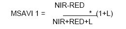
    (20)

    Here, L: 1 - 2*s*NDVI*WDVI, s: slope of the soil line, NDVI: Normalized Difference Vegetation Index, WDVI:  Weighted Difference Vegetation Index, 2: Used to increase the L dynamic range, range of L  = zero to one.

18. Modified Soil-Adjusted Vegetation Index 2 (MSAVI2) : MSVI2 was derived based on a modification of the L factor of the SAVI (Qi, J. et al, 1994). SAVI and MSVI2 are intended to correct the soil background brightness in different vegetation cover conditions. Basically, this is an iterative process and substitute 1-MSAVI (n-1) as the L factor in MSAVI (n) and then inductively solve the iteration where MSAVI (n)=MSAVI (n-1).  MSVI2 uses an inductive L factor to:
    • Remove the soil “ noise “ that was not cancelled out by the product of NDVI by WDVI and
    • Correct values greater than one that MSAVI1 may have due to the low negative value of NDVI*WDVI. Thus its use is limited for high vegetation density areas.

    The general expression of MSAVI2 is,

    MSAVI2= (2NIR +1 - Ö{(2NIR+1)2 – 8(NIR – RED)}) / 2

    (21)

    Where, NIR: reflectance of the near infrared band, RED: reflectance of the red band.

    Pixel value less than 0.0 are under non-vegetation and pixel having greater than 0 are under vegetation.

19. Weighted Difference Vegetation Index (WDVI) : Like PVI, WDVI is very sensitive to atmospheric variations (Richerdson A.J et al, 1977) and can be presented as,
    
    

    WDVI= NIR - gRED

    (22)

    Where, NIR: reflectance of near infrared band, RED: reflectance of visible red band, g: slope of the soil line.

    Although simple, WDVI is as efficient as most of the slope based VI’s. The effect of weighting the red band with the slope of the soil line is the maximization of the vegetation signal in the near-infrared band and the minimization of the effect of soil brightness.

Land use analysis : Classification of remotely sensed data requires the assignment of each of the pixels on an image to a class. The classification approach is based on the assumption that each of the classes on the ground has a class-specific spectral response with each of the classes varying in spectral patterns. There is substantive variation in the distribution of the pixel reflectance values depending upon where the samples are drawn within a land use type (James Campbell, 2002). The spectral information contained in the original and transformed bands is then used to characterise each class pattern, and to discriminate between classes. Both supervised and unsupervised classification approaches were tried to identify land use categories.  In case of supervised classification, known specific types of land-use are identified based on the spectral reflectance patterns or signatures of different features information classes training sites. With these a statistical characterisation of reflectance for each individual class were done, which is known as signature analysis and it may be as simple as the mean or range of reflectance on each band, or as complex as analyses of variance and covariance over all bands. After the signature analysis is done the image is classified by examining the reflectance of each pixel and making a decision about which of the signature it resembles most and assigning the appropriate pixels to their respective class.  Using the information from a set of training sites, Supervised classification was done using Gaussian maximum likelihood classifier (GMLC) to classify the data in to five categories (agriculture, built-up, forest, plantation and waste land). GMLC uses the mean, variance and covariance data of the signatures to estimate a probability that a pixel belongs to each class (Ramachandra, 2007b).

Accuracy Assessment : Accuracy estimation in terms of producer's accuracy, user's accuracy, overall accuracy and Kappa coefficient were subsequently made after generating confusion matrix. The Kappa coefficient is a measure of the difference between the actual agreement between reference data and an automated classifier and the chance agreement between the reference data and the random classifier as shown in equation (1) and equation (2). This statistics serves as an indicator of the extent to which the percentage correct values of an error matrix are due to “true” agreement versus “chance” agreement. It incorporates the non-diagonal elements of the error matrix as a product of the row and column diagonal (Ramachandra, 2007a).

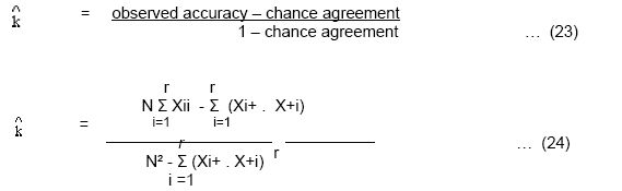
where   r      =    number of rows in the error matrix
            Xii    =   the number of observations in row i and column i (on the major diagonal)
            Xi+   =   total of observations in row i
            X+ i  =   total of observations in column i
            N  =   total number of observations included in matrix